-
Notifications
You must be signed in to change notification settings - Fork 5
/
Copy pathLab06_MaxLike.Rmd
179 lines (117 loc) · 9.92 KB
/
Lab06_MaxLike.Rmd
1
2
3
4
5
6
7
8
9
10
11
12
13
14
15
16
17
18
19
20
21
22
23
24
25
26
27
28
29
30
31
32
33
34
35
36
37
38
39
40
41
42
43
44
45
46
47
48
49
50
51
52
53
54
55
56
57
58
59
60
61
62
63
64
65
66
67
68
69
70
71
72
73
74
75
76
77
78
79
80
81
82
83
84
85
86
87
88
89
90
91
92
93
94
95
96
97
98
99
100
101
102
103
104
105
106
107
108
109
110
111
112
113
114
115
116
117
118
119
120
121
122
123
124
125
126
127
128
129
130
131
132
133
134
135
136
137
138
139
140
141
142
143
144
145
146
147
148
149
150
151
152
153
154
155
156
157
158
159
160
161
162
163
164
165
166
167
168
169
170
171
172
173
174
175
176
177
178
179
---
title: "Lab 06 - Maximum Likelihood"
author: "EE 375"
runtime: shiny
output: html_document
---
The goal of this lab is to help you gain some hands-on familiarity with some of the concepts, tools, and techniques involved in Maximum Likelihood. This example will focus on fitting the Farquhar, von Caemmerer, and Berry (1980) photosynthesis model [FvCB model] to leaf-level photosynthetic data. This is a simple, nonlinear model consisting of 3 equations that models net carbon assimilation, $A^{(m)}$, at the scale of an individual leaf as a function of light and CO2.
$$A_j = \frac{\alpha Q}{\sqrt{1+(\alpha^2 Q^2)/(Jmax^2)}} \frac{C_i- \Gamma}{4 C_i + 8 \Gamma}$$
$$A_c = V_{c,max} \frac{C_i - \Gamma}{C_i+ K_C (1+[O]/K_O) }$$
$$A^{(m)} = min(A_j,A_c) - r$$
The first equation $A_j$ describes the RUBP-regeneration limited case. In this equation the first fraction is a nonrectangular hyperbola predicting $J$, the electron transport rate, as a function of incident light $Q$, quantum yield $\alpha$, and the asymptotic saturation of $J$ at high light $J_{max}$. The second equation, $A_c$, describes the Rubisco limited case, which is a function of $C_i$, the internal CO2 concentration of the leaf. The third equation says that the overall net assimilation, A, is determined by whichever of the two above cases is most limiting, minus the leaf respiration rate, $r$. The superscript _m_ is used to indicate this is a modeled value, while the superscript _o_ will be used to designate the corresponding observed data.
To keep things simpler, today we will focus just on the CO2 limited (i.e. Rubisco) case and combine the last two equations in order to predict **net** photosynthesis.
$$A^{(m)} = V_{c,max} \frac{C_i - \Gamma}{C_i+ K_C (1+[O]/K_O) } - r$$
Furthermore, the term $K_C (1+[O]/K_O)$ only depends on the Oxygen concentration in the atmosphere, which is essentially constant at 20.95%, and so we will simplify this term to the single constant $K_M$ giving us our final model
$$A^{(m)} = V_{c,max} \frac{C_i - \Gamma}{C_i+ K_M} - r$$
Table 1: FvCB model parameters in the statistical code, their symbols in equations, and definitions
Parameter | Symbol | Definition
----------|------------|-----------
cp | $\Gamma$ | CO2 compensation point
Vcmax | $V_{c,max}$ | maximum Rubisco capacity
r | $R_d$ | leaf respiration
Ci | $C_i$ | internal CO2 concentration
K | $K_M$ | half-saturation
sigma | $\sigma$ | residual standard deviation
## Loading the data & exploratory analysis
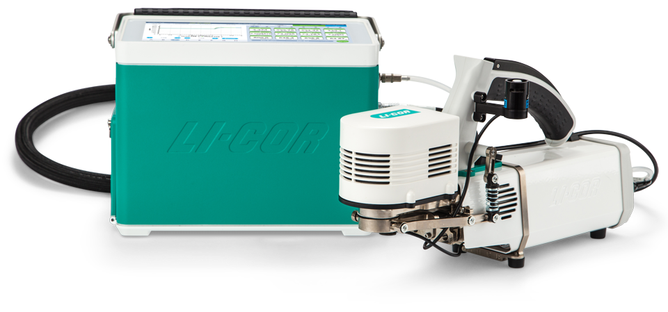
To begin with we'll load up an example A-Ci curve that was collected on an aspen (_Populus tremuloides_) leaf during the [Flux Course](http://www.fluxcourse.org/) at Niwot Ridge. A-Ci curves are generated by placing a leaf in a sealed chamber and measuring the photosynthetic rate as the CO2 concentration is varied. Measurements are made using the same type of infrared laser that is used on flux towers.
The code below reads in the data from this instrument and extracts the variables we need (Ci, Ca, Ao).
```{r}
##' @name read.Licor
##' @author Mike Dietze
##' @param filename name of the file to read
##' @param sep file delimiter. defaults to tab
##' @param ... optional arguments forwarded to read.table
read.Licor <- function(filename,sep="\t",...){
fbase = sub(".txt","",tail(unlist(strsplit(filename,"/")),n=1))
print(fbase)
full = readLines(filename)
## remove meta=data
start = grep(pattern="OPEN",full)
skip = grep(pattern="STARTOFDATA",full)
for(i in length(start):1){
full = full[-(start[i]:(skip[i]+1*(i>1)))] # +1 is to deal with second header
}
full = full[grep("\t",full)] ## skip timestamp lines
dat = read.table(textConnection(full),header = TRUE,blank.lines.skip=TRUE,sep=sep,...)
fname=rep(fbase,nrow(dat))
dat = as.data.frame(cbind(fname,dat))
return(dat)
}
## Load the data
dat <- read.Licor("flux-course-3aci")
## grab the variables we need
Ci = dat$Ci ## CO2 concentration in the leaf
Ca = dat$CO2R ## CO2 concentration in the chamber
Ao = dat$Photo ## Observed net Assimilation (photosynthetic rate)
## sort the data in order for convenience
ord = order(Ci)
Ci = Ci[ord]
Ca = Ca[ord]
Ao = Ao[ord]
```
### Question 1
Make a plot of $A^{(o)}$ as a function of $C_i$ ($A^{(o)}$ on Y axis and $C_i$ on x axis).
## FvCB model
Next, let's code up the FvCB model as a function. In the version below I've passed two arguments, a vector of parameters (theta), and Ci. I then extract the variables I need from this vector and perform the calculation
```{r}
FvCB <- function(theta,Ci){
Vcmax = theta[1]
K = theta[2]
cp = theta[3]
r = theta[4]
Anet = Vcmax*(Ci-cp)/(Ci+K) - r
return(Anet)
}
```
### Question 2
*(A)* Using Shiny, make an interactive plot that shows both the data and the model. Specifically, create sliders for the model parameters, param = c(Vcmax,K,cp,r,sigma). Then, to add the curve to your previous plot, you'll want to create a sequence of Ci values and feed this and your parameters to the FvCB function to calculate the mean prediction at each Ci. When setting the allowable ranges for parameters
* Vcmax has to be positive and can be larger than the highest observed value on the y-axis, but usually not by a lot.
* K and cp can take on any value across the range of the x-axis, though in practice cp is usually less than K
* r has to be positive but is unlikely to be more than 10% of Vcmax
Hint: Don't start from scratch! It's fine to copy, paste, and modify your Lab 3 code for drawing a straight line through data. Also remember to add complexity one step at a time. For example, it's fine to start with getting your old code to draw a straight line through this new data, and then one at a time add new parameters to the model and new sliders for those parameters, checking to make sure things work at eachstep.
*Extra Credit:* To approximate the uncertainty (in terms of a 95% predictive interval), you'll also want to add additional lines 1.96*sigma above and below the mean lines (e.g. with a different line type or color).
*(B)* Using your Shiny app, figure out a sensible initial guess for the value of the model parameters, param = c(Vcmax,K,cp,r,sigma). Note, the goal of this isn't to guess the 'right' parameter values, or to spend a lot of time hand tuning the parameters, since Maximum Likelihood will do that for you with much greater speed, precision, and statistical rigor. The primary goal is to make sure you have some understanding of the parameters of the model and what they control. The secondary goal is to get the initial guess in the right ballpark (e.g., so the plot is on the same page as the data).
## Fitting the model
As a Likelihood we'll assume that the observed leaf-level assimilation $A^{(o)}$ is Normally distributed around the model predictions with observation error $\sigma^2$.
$$A^{(o)} \sim N(A^{(m)},\sigma^2)$$
To fit this model to data we'll have to define a Likelihood function that combines our process model with our Likelihood. Furthermore, since we know the thing that we want to do is to minimize the negative log likelihood, we'll go ahead and include the log and the sign change in the function.
```{r}
lnLike <- function(theta,Ao,Ci){
sigma = theta[5]
## write code here that calculates the log Likelihood, use the FvCB to calculate the mean
return(-lnL)
}
```
### Question 3
Evaluate your lnLike function given your initial parameter guess, and the observed $A^{(o)}$ and $C_i$. i.e. plug these things into your new function and report the single number that comes out. If you get something non-sensible that's not a number (e.g. NA, NAN, Inf) you either have a bug in your code, or a poor initial guess, and need to try again before moving on to question 4.
### Question 4
Use the function _optim_ to minimize the negative log Likelihood (i.e. to maximize the Likelihood). Don't forget to pass the additional arguments to lnLike *by name* (i.e. Ao=Ao,Ci=Ci ) within the optim function call. Save the output from optim to a variable _fit_. Report **and explain** the contents of _fit_.
## Evaluating the model
### Question 5
Run the FvCB model with your best fit parameters and save the results to the variable _Am_.
Repeat your plot of the observed data, but this time add lines for the best fit model.
### Question 6
Generate a predicted vs observed plot and include a 1:1 line (a plot that includes a line with an intercept of 0 and a slope of 1). Also include the diagnostic regression line between the predicted and observed and save the output of this _lm_ to the variable 'bias.fit'. Make sure to include a legend indicating which line is which.
*Overall, how did the model perform?*
### Question 7
An important thing to note about the bias fit regression line is that the standard regression F-test, which assesses deviations from 0, is not the test you are actually interested in, which is whether the line differs from 1:1. Therefore, while the test on the intercept is correct, as this value should be 0 in an unbiased model, the test statistic on the slope is typically of less interest (unless your question really is about whether the model is doing better than random). However, this form of bias can easily be assessed by looking to see if the CI for the slope overlaps with 1.
Use the function _confint_ to determine whether the bias.fit model is different from the 1:1 line.
Report the $R^2$ and RMSE of the model.
Compare the RMSE to the best fit parameter sigma.
### Question 8
Use your standard residual diagnostic plots, applied to bias.fit, to assess to what extent the model meets the assumptions we made (no trend in residuals, Normal distributed error, constant variance)
### Extra Credit
What is the most abundant protein on Earth? How does this relate to your findings in this lab?
## Citations
Farquhar, G., Caemmerer, S. & Berry, J.A. (1980). A biochemical model of photosynthetic CO2 assimilation in leaves of C3 species. Planta, 149, 78–90.