-
Notifications
You must be signed in to change notification settings - Fork 12
ExampleForecast
The following section details the process of developing forecast equations for Inflows into Gibson Reservoir, near Augusta, MT. Gibson Reservoir is located at the confluence of the North Fork and South Fork Sun River on the Front Range of Montana. Inflow is primarily from snowmelt runoff and spring/early summer upslope precipitation. No depletions exist upstream of Gibson Reservoir. Much of the basin is within the Bob Marshall Wilderness, leaving us few point measurements of snowpack, precipitation, and air temperature within the basin.
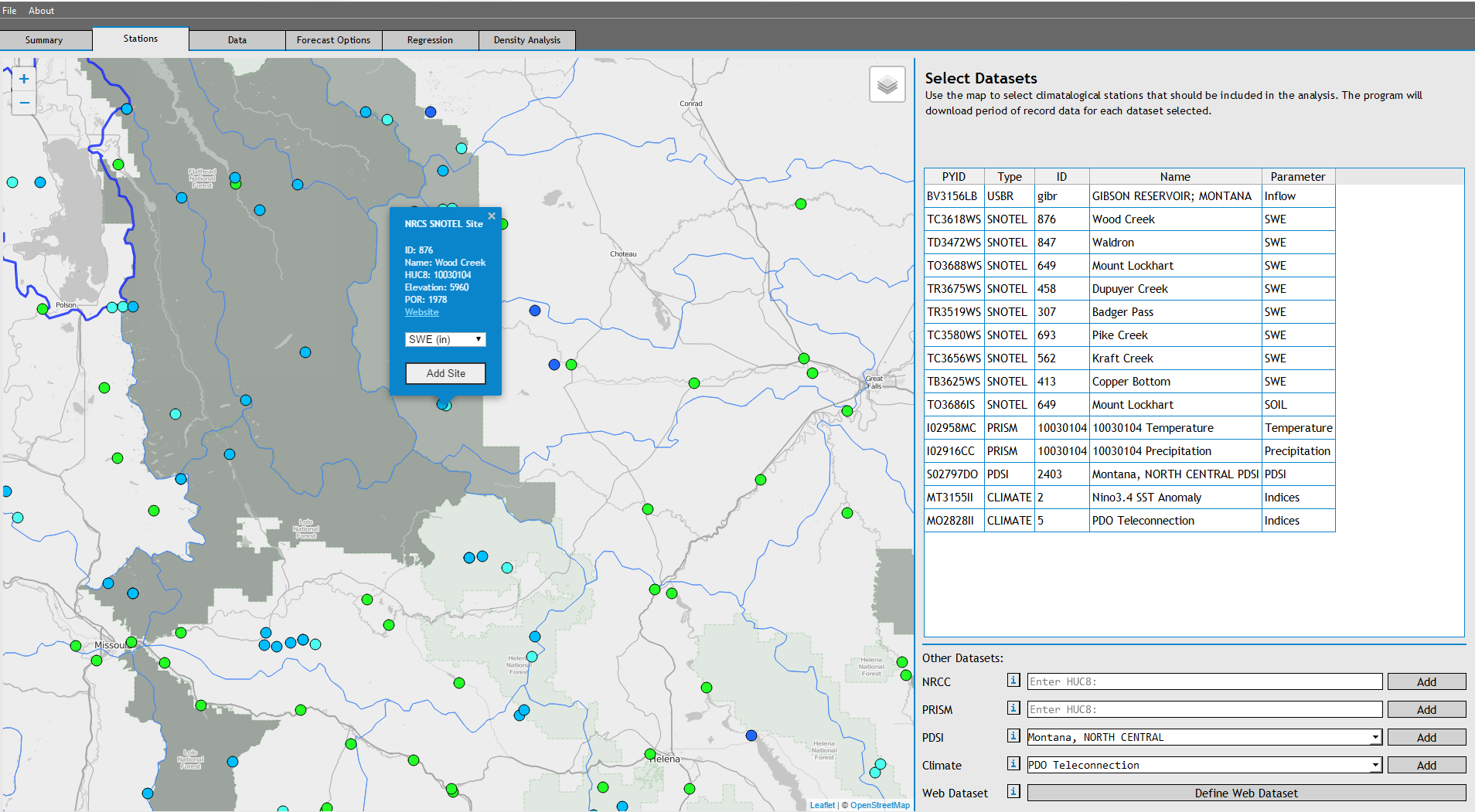
We'll begin the forecast development by finding relevant datasets using the Stations Tab.
Use the map to navigate the to Sun Basin, which is directly west of Augusta, MT.
Using the map markers, add the USBR station GIBSON RESERVOIR. Select nearby SNOTEL stations and add them to the Stations List. Additionally, add the PRISM data for HUC 10030104, and the Nino3.4 SST Anomaly Dataset. When stations are selected, the program automatically assigns them a 'PYID' and saves thier metadata internally. If you wanted to define a custom dataset using a user-defined dataloader, you could define it on this Tab.
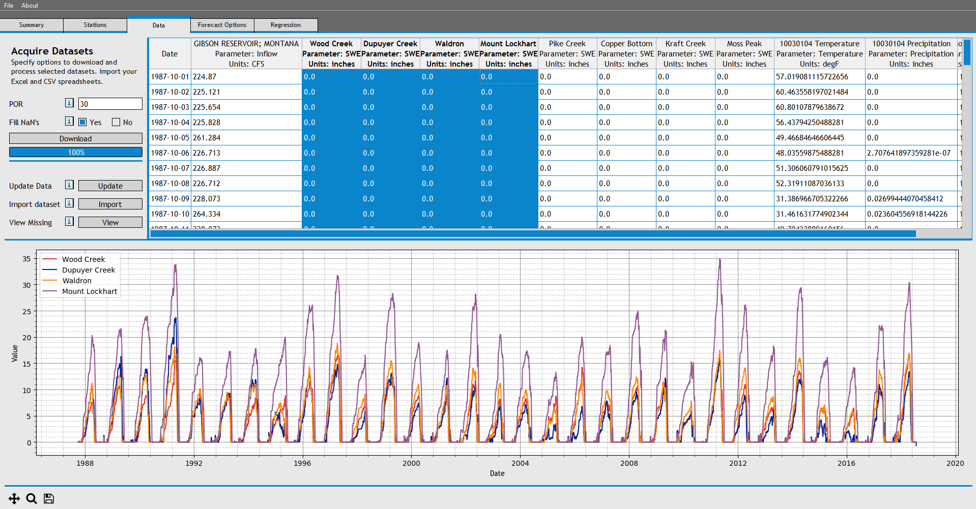
Next, download the data for the datasets we selected. Navigate to the Data Tab, and download 30 years of data.
We now have 30 years of daily data for each dataset we specified in the stations tab.
Once the data is downloaded, click on the column headers (one or multiple) to view individual datasets. We can also view the serial completeness of our downloaded data by choosing the 'View Missing' button. If your dataset isn't missing too much data, continue on to the next section.
Users have the option to manually correct or insert any values into the dataset at this point. Entire datasets can be deleted by right clicking on the column names if they don't meet the users standards for inclusion.
If you wanted to import a flat file as a dataset, you would do that here using the 'Import Dataset' button.
Now would also be a good point to save our forecast. Choose 'Save Forecast' from the file menu.
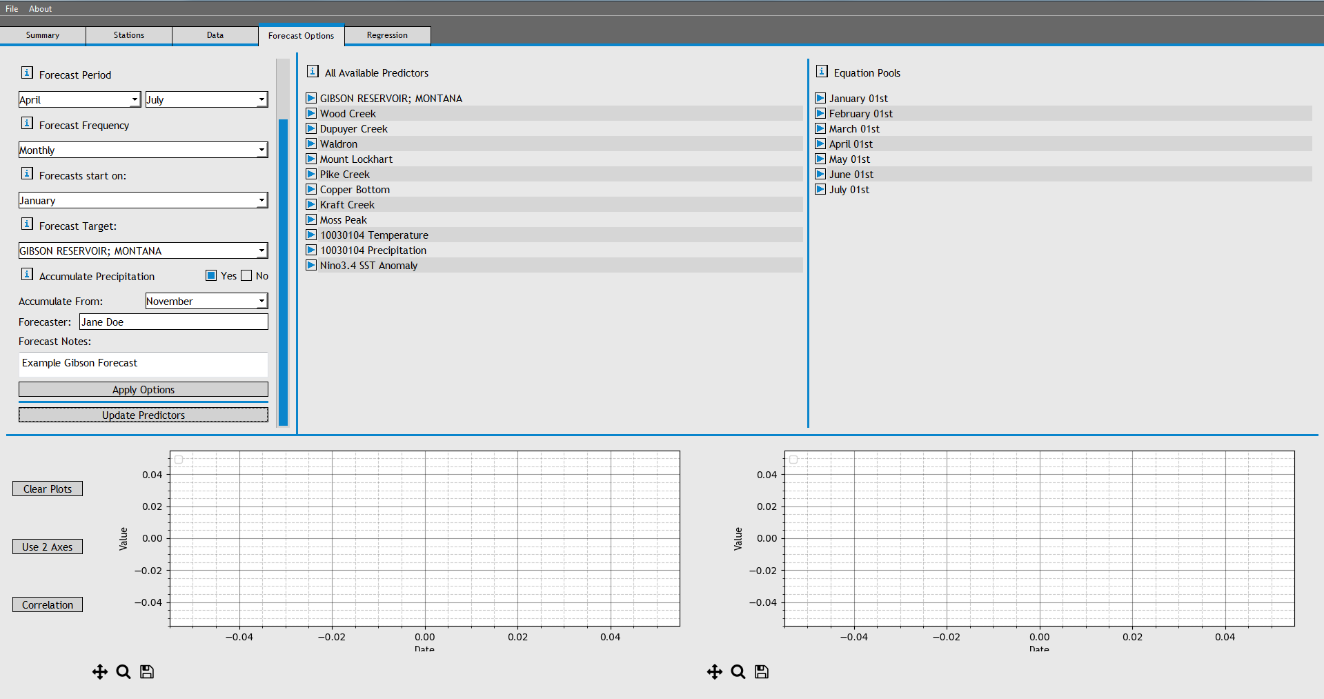
Now that we have daily data, we can process it into monthly re-sampled predictors. Navigate to the Forecast Options Tab and begin filling out the options in the 'Set Options' pane.
We'll generate April-July forecast equations on a monthly basis, So select a Forecast Period of 'April' through 'July', a forecastfrequency of 'Monthly', and start forecasts in 'January'. Additionally, we'll include an accumulated running total of precipitation from November, so set the 'Accumulate From' drop-down box to 'November'.
Choose 'Apply Options' and wait for the program to generate seasonal predictors. (NOTE: This process has not been optimized yet, so it may be a bit slow).
At this point we have now generated a seasonal predictors for each dataset that we specified in the stations tab. Browse through the seasonal predictors in the 'All Available Predictors' tree. To view a plot of a seasonal predictor, drag it into the plotting window below the tree. You are able to view correlations between 2 predictors if you drag 2 predictors into the plots.
We now need to add potentially relevant predictors to specific forecast equations. At this point, we're just telling the program which predictors to consider when it is developing forecast equations.
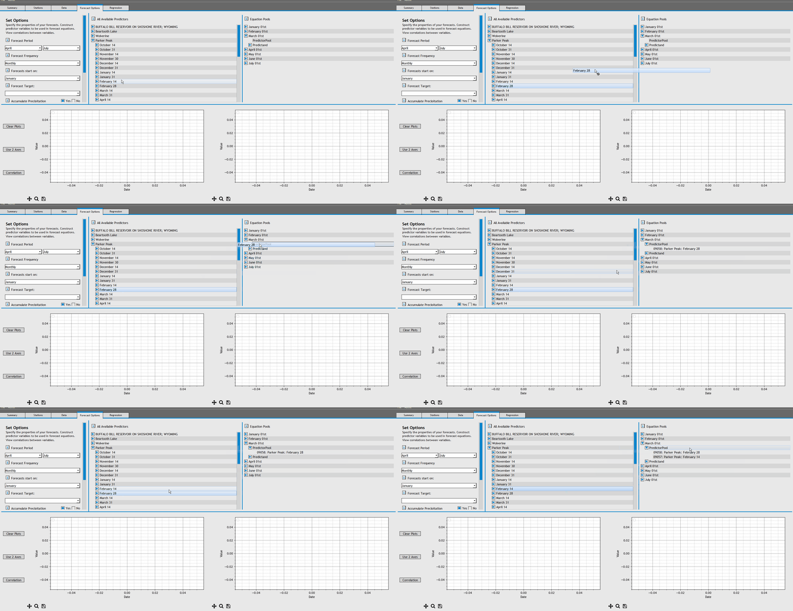
To begin, expand the forecast equation for 'April 01st'. Add the following predictors to the April 01st PredictorPool:
- GIBSON RESERVOIR, MONTANA, November 01-31
- Wood Creek, March 31
- Wood Creek, March 14
- Dupuyer Creek, March 31
- Dupuyer Creek, March 14
- Waldron, March 31
- Waldron, March 14
- Mount Lockhart, March 31
- Mount Lockhart, March 14
- Pike Creek, March 31
- Pike Creek, March 14
- Copper Bottom, March 31
- Copper Bottom, March 14
- Kraft Creek, March 31
- Kraft Creek, March 14
- Moss Peak, March 31
- Moss Peak, March 14
- 10030104 Temperature, March 01- March 31
- 10030104 Temperature, February 01 - February 28
- 10030104 Precipitation, November 01 - March 31
- 10030104 Precipitation, March 01 - March 31
- Nino3.4 SST Anomaly, March 01 - March 31
- Nino3.4 SST Anomaly, February 01- February 28
At this point, save the forecast.
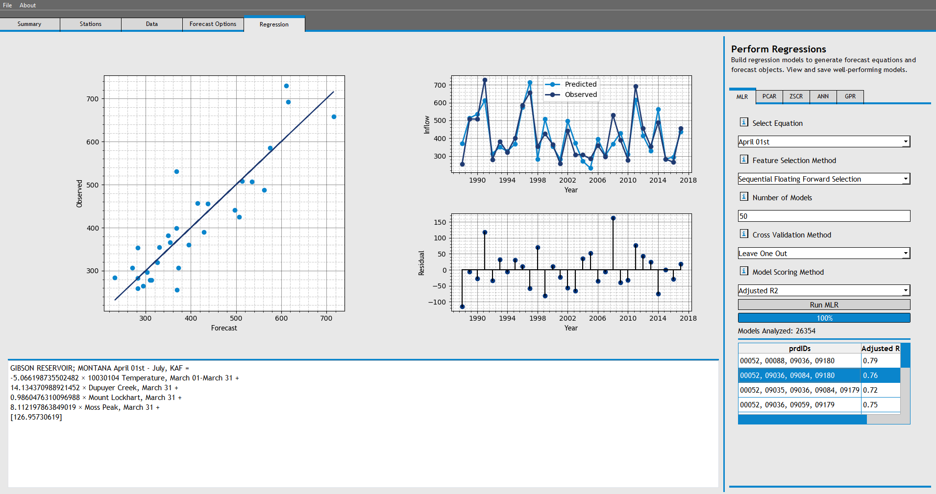
On the Regression Tab, navigate to the MLR tab, and choose 'April 01st' as the equation. Leave all the other options and choose 'Run MLR'.
The program will begin analyzing thousands of models using Sequential Forward Floating Selection, and will return 50 models, each with features chosen for thier impact on model skill.
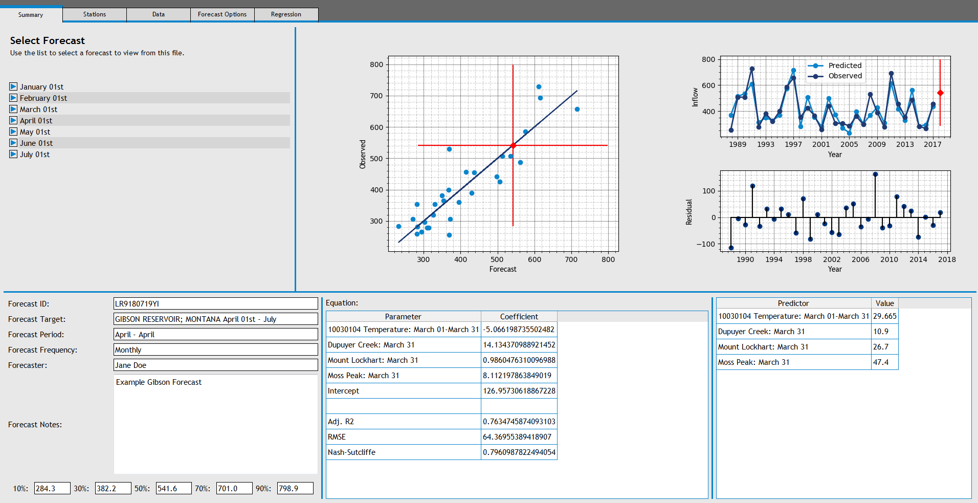
Select a model in the models list to view the forecast equation and model plots. The largest plot displays the correlation between the values predicted by the forecast equation, and the actual observed inflows. The plot on the top-right displays the time series graph of predicted inflow vs observed inflow, with the residuals in the bottom-right plot.
Right click the second forecast in the list and select "Save Forecast".
Users can also generate models using Principal Components Regression or Z-Score Regressions by navigating to the other sub-tabs in the Regression Tab.
Return to the Summary Tab and navigate through the 'April 01st' entry to the Forecast we just saved. Right click on the forecast and choose "Generate Current Forecast". The program will now gather the predictor data for the current year (if it exists) and generate a current water year forecast as well as a prediction interval.
The same procedure of saving forecasts can be repeated for other regression equations developed in the Regression Tab.
If you have more than one forecast that you want to compare, navigate to the Density Analysis tab and select the month of the forecast equations you want to analyze. In this case, if you generated multiple April 1st forecasts, select 'April' from the drop-down list in the top left corner of the tab. Next highlight all the forecasts that you would like to compare in the forecast list and choose 'Run Analysis'. The software will perform a Kernel Density Estimation and return a composite forecast density function, that can then be used to retrieve the non-exceedance values.
When the user selects the 'Run Analysis' button, the software generates a normal distribution for each forecast selected. The normal distriubtion for each forecast is defined with the mean equal to the 50% exceedance value and the standard deviation equal to the [(90% value - 50% value) / 1.28]. This effectively describes a normal distribution which mirrors the mean and uncertainty of the individual forecast. Next, the software randomly samples 1000 points from each normal distribution. If you're analyzing 10 forecasts, the software now has 10,000 randomly sampled forecasts. The software then takes these 10,000 randomly sampled points and uses a kernel density estimation convolution to draw a new forecast distribution.
