Installation Guide | readthedocs | What is CTI?
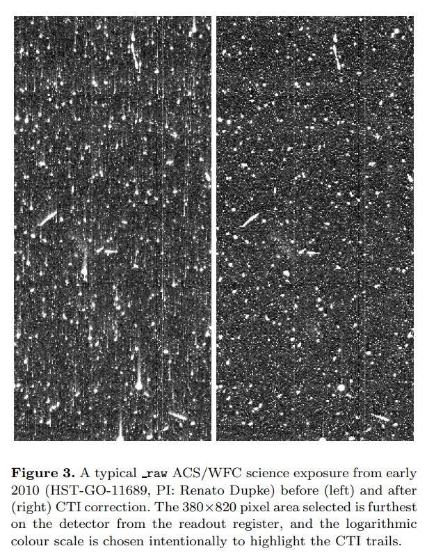
Charge Transfer Inefficiency, or CTI for short, is an effect that occurs when acquiring imaging data from Charge Coupled Devices (CCDs). Due to radiation damage to the CCD's silicon lattice electrons are read-out inefficiently, creating a characteristic trailing or smearing effect.
Here is an example of CTI in the Hubble space telescope, after decades of radiation damage:
PyAutoCTI makes it simple to calibrate a time-varying CTI model using in-orbit observations and correct CTI in science imaging using this model.
PyAutoCTI development is centred around mitigating CTI for the Euclid space mission, which relies on the precise measurement of galaxy shapes in order to map out the distribution of dark matter throughout the Universe via a phenomena called weak gravitational lensing.
The following links are useful for new starters:
- The PyAutoCTI readthedocs, which includes an installation guide and an overview of PyAutoCTI's core features.
- The autocti_workspace GitHub repository, which includes example scripts.
To model CTI, PyAutoCTI wraps the library arCTIc (https://github.com/jkeger/arctic).
CTI can be added to an image as follows:
import autocti as ac

"""
Define a pre-cti image which **PyAutoCTI** adds CTI to.
"""
pre_cti_data_2d = ac.Array2D.no_mask(
            values=[
        [0.0, 0.0, 0.0, 0.0, 0.0, 0.0, 0.0, 0.0],
        [0.0, 10.0, 10.0, 10.0, 0.0, 0.0, 0.0, 0.0],
        [0.0, 10.0, 10.0, 10.0, 0.0, 0.0, 0.0, 0.0],
        [0.0, 10.0, 10.0, 10.0, 0.0, 0.0, 0.0, 0.0],
        [0.0, 0.0, 0.0, 0.0, 0.0, 0.0, 0.0, 0.0],
        [0.0, 0.0, 0.0, 0.0, 0.0, 0.0, 0.0, 0.0],
        [0.0, 0.0, 0.0, 0.0, 0.0, 0.0, 0.0, 0.0],
        [0.0, 0.0, 0.0, 0.0, 0.0, 0.0, 0.0, 0.0],
        [0.0, 0.0, 0.0, 0.0, 0.0, 0.0, 0.0, 0.0],
        [0.0, 0.0, 0.0, 0.0, 0.0, 0.0, 0.0, 0.0],
    ],
    pixel_scales=0.1,
)

"""
A clocker object is used to model CCD clocking, which includes customization such
as the properties of the read-out electronics.
"""
clocker_2d = ac.Clocker2D(parallel_roe=ac.ROE())

"""
CTI is caused by traps on the CCD's silicon lattice, for example traps which capture
electrons instantaneously.
"""
parallel_trap = ac.TrapInstantCapture(density=100.0, release_timescale=1.0)

"""
CTI also depends on how electrons fill each pixel in a CCD, therefore we define
the volume-filling properties of the CCD.
"""
parallel_ccd = ac.CCDPhase(
    well_fill_power=0.58, well_notch_depth=0.0, full_well_depth=200000.0
)

"""
The data, traps and CCD properties are combined to clock the pre-CTI data and return the
post-CTI data.
"""
post_cti_data_2d = clocker_2d.add_cti(
    data=pre_cti_data_2d,
    parallel_trap_list=[parallel_trap],
    parallel_ccd=parallel_ccd
)

"""
We can use PyAutoCTI's built in visualization library to plot the data with CTI.
"""
import autocti.plot as aplt

array_2d_plotter = aplt.Array2DPlotterarray=post_cti_data_2d)
array_2d_plotter.figure_2d()
With PyAutoCTI, you can begin calibrating a CTI model in minutes. The example below demonstrates a simple analysis which fits a CTI model to charge injection imaging calibrate data (a form of data used to calibrate a CTI model)
import autofit as af
import autocti as al
import autocti.plot as aplt

"""
Define the 2D shape of the charge injection image.
"""
shape_native = (30, 30)

"""
Define where the charge injection is on the data.
"""
regions_list = [(0, 25, serial_prescan[3], serial_overscan[2])]

"""
Setup the data layout which informs **PyAutoCTI** where information on
CTI is in the data.
"""
layout = ac.Layout2DCI(
    shape_2d=shape_native,
    region_list=regions_list,
)

"""
Load the charge injection image from fits.
"""
dataset = ac.ImagingCI.from_fits(
    data_path=path.join(dataset_path, f"data.fits"),
    noise_map_path=path.join(dataset_path, f"noise_map.fits"),
    pre_cti_data_path=path.join(dataset_path, f"pre_cti_data.fits"),
    layout=layout,
    pixel_scales=0.1,
)

"""
Again define the clocker which models CCD clocking and read-out electronics.
"""
clocker_2d = ac.Clocker2D(parallel_roe=ac.ROE())

"""
Define the traps in the CTI model and customize the priors of their free parameters.
"""
trap = af.Model(ac.TrapInstantCapture)

trap.density = af.UniformPrior(lower_limit=0.0, upper_limit=20.0)
trap.release_timescale = af.UniformPrior(lower_limit=0.0, upper_limit=20.0)

"""
Define the CCD filling behaviour of the CTI, which is also part of the model and is
fitted for as free parameters.
"""
parallel_ccd = af.Model(ac.CCDPhase)

parallel_ccd.well_fill_power = af.UniformPrior(lower_limit=0.0, upper_limit=1.0)
parallel_ccd.well_notch_depth = 0.0
parallel_ccd.full_well_depth = 200000.0

"""
We define the non-linear search used to fit the model to the data (in this case, Dynesty).
"""
search = af.Nautilus(name="search[example]", n_live=50)

"""
We next set up the `Analysis`, which contains the `log likelihood function` that the
non-linear search calls to fit the cti model to the data.
"""
analysis = ac.AnalysisImagingCI(dataset=dataset, clocker=clocker_2d)

"""
To perform the model-fit we pass the model and analysis to the search's fit method. This will
output results (e.g., dynesty samples, model parameters, visualization) to hard-disk.
"""
result = search.fit(model=model, analysis=analysis)

"""
The results contain information on the fit, for example the maximum likelihood
model from the Dynesty parameter space search.
"""
print(result.samples.max_log_likelihood())
Support for installation issues, help with cti modeling and using PyAutoCTI is available by raising an issue on the GitHub issues page.
We also offer support on the PyAutoCTI Slack channel, where we also provide the latest updates on PyAutoCTI. Slack is invitation-only, so if you'd like to join send an email requesting an invite.


