APF
APF is based on an object moving under the effect of potential fields. The potential field exerts a force on the bot which allows the bot to move. The net field acting on the bot is the summation of attractive field of destination point and repulsive field of the obstacles. The path is computed using gradient descent algorithm which moves the bot in the direction of decreasing field.
Main challenge with this approach is the problem of local minima.
1. Use of gaussian function for source , obstacles and destination
● The idea is to generate peaks at the location of obstacles and sink at the goal by making use of the gaussian function. The gradient of which can be used such that the peaks serves a repulsive potential field near the obstacle which let the bot to move away from it. And the sink would serve as a attractive potential field at the goal which makes the bot to move towards the goal.
● Consider a circular Gaussian Function, having a bivariate normal distribution and equal standard deviation i.e.


● Let x1 , y1 be the coordinates of a point where source , obstacle or goal is located. To generate a gaussian surface considering any of the above as its centre, use the
Following in the above gaussian function:
-
Exponent=
-
Amplitude =


And for the sink amplitude will be the negative of the above.
● Following are some test cases performed using the above function:
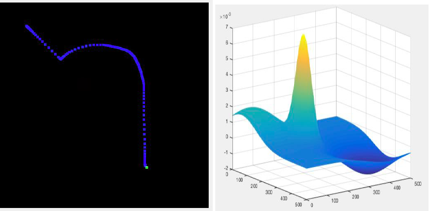
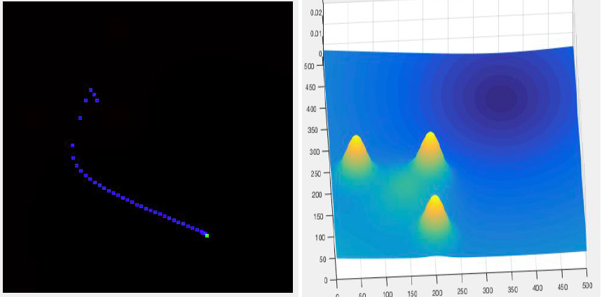
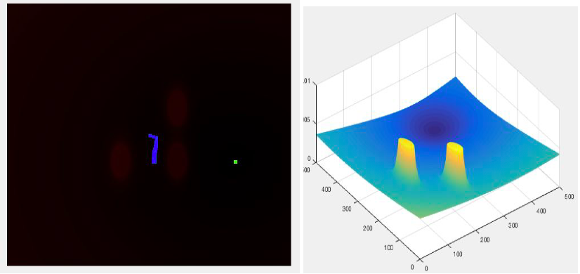
● In the cases below , the image at the left depict the path of the bot , and the right one shows the map of the potential field generated using the gaussian function
● The green point represents the destination point in the left image
● Consider a map of size 500 x 500
Case 1:
| POINT | LOCATION | SIGMA VALUE |
|---|---|---|
| Obstacle | 200, 200 | 30 |
| Initial | 55, 62 | 100 |
| Final | 400, 350 | 100 |
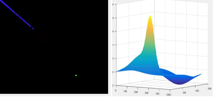
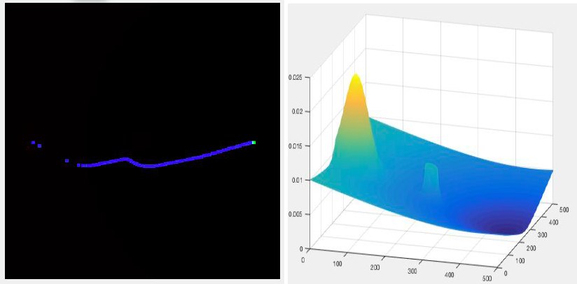
Case 2:
| POINT | LOCATION | SIGMA VALUE |
|---|---|---|
| Obstacle | 200, 200 | 50 |
| Initial | 55, 62 | 100 |
| Final | 400, 350 | 100 |

Observation : As sigma value of obstacle is increased, the path takes a bigger round near obstacle and then stops due to the absence of potential Gradient nearby
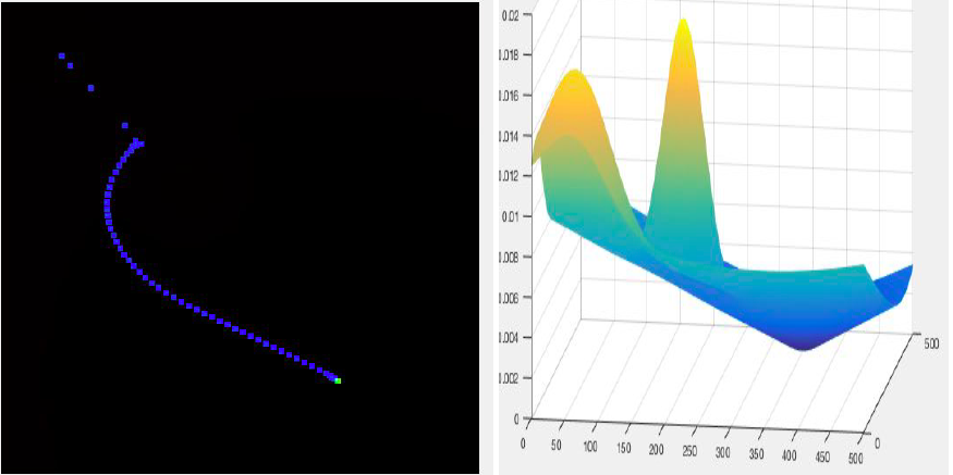
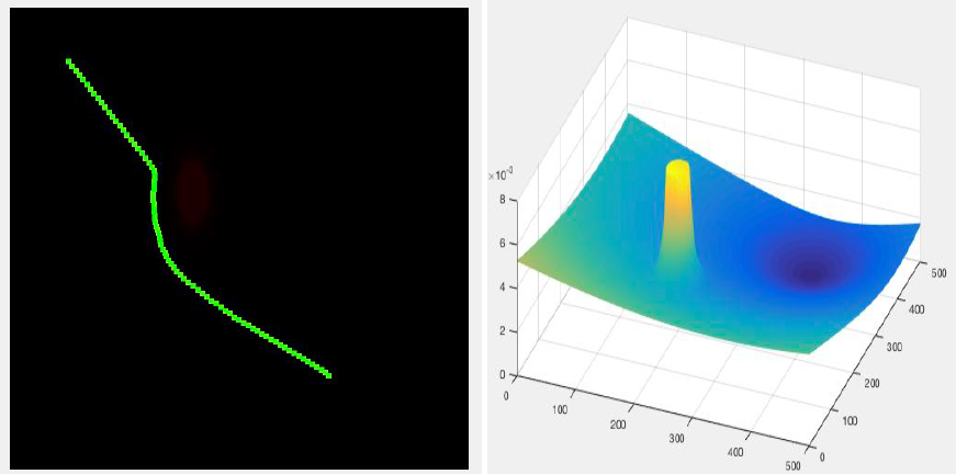
Case 3: When obstacle is near to the initial point
Observation:
-
The gaussian peak surface of source and obstacle merges with each other as they are close.
-
As by the map, the lower gradient is at the back side of source , the bot moves away from the destination
-
To reach the destination sigma of the destination point must be sufficiently larger.
| POINT | LOCATION | SIGMA VALUE |
|---|---|---|
| Obstacle | 200, 200 | 30 |
| Initial | 150, 150 | 80 |
| Final | 400, 350 | 100 |
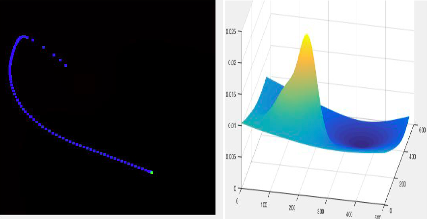
2. Use of parabolic function for the goal instead of gaussian function
● In search of better results , we switched to a parabolic attractive field function from the gaussian function for the goal point as given below:
● Here the net potential field is the sum of the gaussian function for obstacles and source and the parabolic function for goal


Case 1:
| POINT | LOCATION | SIGMA VALUE |
|---|---|---|
| Obstacle | 200, 200 | 30 |
| Initial | 55, 62 | 50 |
| Final | 400, 350 | 150 |
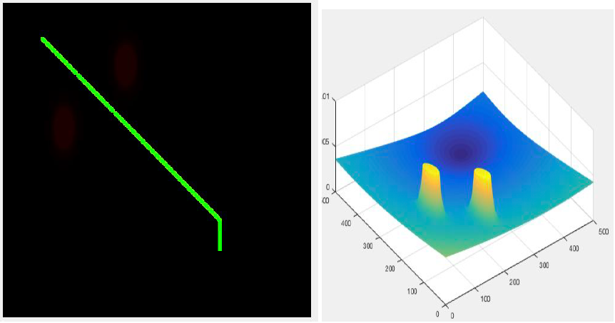
Case 2: When obstacle is near to the source
| POINT | LOCATION | SIGMA VALUE |
|---|---|---|
| Obstacle | 200, 200 | 30 |
| Initial | 150, 150 | 50 |
| Final | 400, 350 | 150 |
Observation: Here, when the gaussian function for the goal is changed to the parabolic one,bot successfully gets a path towards the goal, unlike the gaussian function case
Case 3:
| POINT | LOCATION | SIGMA VALUE |
|---|---|---|
| Obstacle 1 | 200, 50 | 30 |
| Obstacle 2 | 200, 200 | 30 |
| Obstacle 3 | 50, 200 | 30 |
| Initial | 150, 150 | 50 |
| Final | 400, 350 | 150 |
 Observation: Bot stops in between
Case 4: On decreasing sigma of the obstacle in the above case
| POINT | LOCATION | SIGMA VALUE |
|---|---|---|
| Obstacle 1 | 200, 50 | 20 |
| Obstacle 2 | 200, 200 | 20 |
| Obstacle 3 | 50, 200 | 20 |
| Initial | 150, 150 | 50 |
| Final | 400, 350 | 150 |
 Observation : This time it works, bot gets a path to reach the goal
3. Use of plateau function for the obstacles instead of gaussian :
Following function is used for the obstacle repulsive potential instead of the gaussian:

where, 

Case 1:
| POINT | LOCATION | SIGMA VALUE |
|---|---|---|
| Obstacle 1 | 250, 250 | 20 |
| Initial | 250, 50 | 30 |
| Final | 250, 450 | 150 |
Observation: Bot not moves from the initial point as the gradient along the rectangular axes is same
Case 2: Same case as above, but now instead of checking the gradient only along the rectangular axes , it is checked in all possible radial directions
4. Remove any repulsive potential field for the source:
As we have considered a parabolic function for the goal point the bot automatically moves away from the source.
5. Ignore consideration of sigma for any point
6. Use of a filter waypoint function to make the path smooth :
The code first find the appropriate path then this filter waypoint function ,by the use of a list , takes the consecutive three points successively. And check the gradient at the mid-point of the first and third point, if it is less than the gradient of the second point, the second point is changed by the mid point. In this way, the function iteratively check for the points until the path becomes smooth.
Consider a = 100 ,b = 50
Case 1: One obstacle
| POINT | LOCATION |
|---|---|
| Obstacle 1 | 200, 200 |
| Initial | 55, 62 |
| Final | 400, 350 |
Case 2: Two obstacles
| POINT | LOCATION |
|---|---|
| Obstacle 1 | 200, 150 |
| Obstacle 2 | 300, 300 |
| Initial | 55, 62 |
| Final | 400, 350 |

Case 3:
| POINT | LOCATION |
|---|---|
| Obstacle 1 | 200, 100 |
| Obstacle 2 | 100, 200 |
| Initial | 55, 62 |
| Final | 400, 350 |
Case 4: Three obstacles
| POINT | LOCATION |
|---|---|
| Obstacle 1 | 200, 300 |
| Obstacle 2 | 300, 300 |
| Obstacle 3 | 300, 200 |
| Initial | 250, 250 |
| Final | 300, 400 |
Observation: Failed to find a path, when the goal is present at the back of the obstacle
Case 5:
| POINT | LOCATION |
|---|---|
| Obstacle 1 | 150, 300 |
| Obstacle 2 | 150, 150 |
| Obstacle 3 | 350, 225 |
| Initial | 250, 50 |
| Final | 250, 450 |
