6 Functions

6.1 Introduction

This section outlines many subjects related to functions, their

Components
Syntax
Scoping Rules
Argument Evaluation
Exit Handlers

6.2 Function Fundamentals

6.2.1 Function Components

To understand functions in R we need to consider two important ideas. First, functions are objects just as vectors are. Secondly, a function whichever she is can be broken into three components.

Arguments formals()
Body body()
environment environment()

Notation

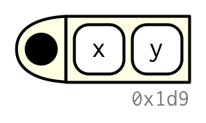
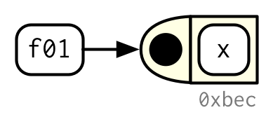
For the rest of this wiki (and as it is in the book), we are gonna use the following notation for functions. The black dot on the left is the function environment and the two blocks to the right are the function arguments. The body of the function is often large and not useful for the sake of the explanation of the topics covered here.

Even though it is possible to print the body of a function with body(), it is more useful to print the function body via the attribute srcref using attr(f, "srcref") because this way of printing does not omit function comments and other formatting.

6.2.2 Primitive Functions

Primitive functions are R functions written in C code. Consequently, these functions are the only ones that do not follow the rules of the three components of common R functions. Examples of primitive functions are sum and [:

formals(sum)
#> NULL
body(sum)
#> NULL
environment(sum)
#> NULL

They have either the type builtin or special:

sum
#> function (..., na.rm = FALSE)  .Primitive("sum")
`[`
#> .Primitive("[")

typeof(sum)
#> [1] "builtin"
typeof(`[`)
#> [1] "special"

6.2.3 First-class Functions

It is important to keep in mind that R functions are simply objects. Therefore, the binding procedure is the same as for any other R object. This is a language property often called first-class functions.

the functions that are not bound to a name are called anonymous functions. They are useful when the name itself won't be need when using the function:

lapply(mtcars, function(x) length(unique(x)))

6.2.4 Invoking Functions

Often, a function is called by passing its parameters directly as in mean(1:10, na.rm = TRUE). However, it is possible to save the arguments in a data structure such as a list and call the function using do.call:

args <- list(1:10, na.rm = TRUE)

do.call(mean, args)
#> [1] 5.5

Extras

The functions is.function and is.primitive returns if an object is a function, a primitive or neither.
the function match.fun lets you find a name is bound to a function, e. g. match.fun("mean").
When does printing a function not show what environment it was created in? Primitive functions and functions created in the global environment do not print their environment.

6.3 Function composition

There are multiple ways of stacking function calls. One can either

Nest function calls, f(g(x)), is concise, and well suited for short sequences. But longer sequences are hard to read because they are read inside out and right to left.
Intermediate objects, y <- f(x); g(y), requires you to name intermediate objects. This is a strength when objects are important, but a weakness when values are truly intermediate.
Piping, x %>% f() %>% g(), allows you to read code in straightforward left-to-right fashion and doesn’t require you to name intermediate objects. But you can only use it with linear sequences of transformations of a single object. It also requires an additional third-party package (magrittyr) and assumes that the reader understands piping.

6.4 Lexical Scoping

Scoping is the act of finding the value associated with a name (i.e. finding the value of an object bound to a name).

R uses lexical scoping: it looks up the values of names based on how a function is defined, not how it is called. It's a technical CS term that tells us that the scoping rules use a parse-time, rather than a run-time structure.

The primary rules of lexical scoping in R are:

Name Masking: Names defined inside a function mask names defined outside a function.
Functions versus Variables: Functions are essentially R objects, this implies that the name masking rules also holds for them.
A Fresh Start: Every time a function is called a new environment is created to host its execution. This means that a function has no way to tell what happened the last time it was run; each invocation is completely independent.
Dynamic Lookup: R looks for values when the function is run, not when the function is created.

6.4.1 Name Masking

When R runs a function, it needs to identify which objects are bound to the names used in the function. First, R looks inside the current function that is being executed for an occurrence of the names it founds and are necessary to perform calculations. Then, it looks where that function was defined (and so on, all the way up to the global environment). Finally, it looks in other loaded packages.

x <- 1
g04 <- function() {
  y <- 2
  i <- function() {
    z <- 3
    c(x, y, z)
  }
  i()
}
g04()
#> [1] 1 2 3

6.4.2 Functions versus Variables

R lexical scoping rules for functions work almost the same way as for objects (after all, R functions are objects). However, when a function and a non-functions share the same name (they must, of course, reside in different environments), applying these rules gets a little more complicated. For example, g09 takes on two different values:

g09 <- function(x) x + 100
g10 <- function() {
  g09 <- 10
  g09(g09)
}
g10()
#> [1] 110

6.4.3 A Fresh Start

The principle of the fresh start states that whenever a function is run, it does not relies on the previous executions of that function. This implies that it is not possible to recycle objects values among function calls. An example of that is the following code:

g11 <- function() {
  if (!exists("a")) {
    a <- 1
  } else {
    a <- a + 1
  }
  a
}

g11()
#> [1] 1
g11()
#> [1] 1

This happens because every time a function is called a new environment is created to host its execution. This means that a function has no way to tell what happened the last time it was run; each invocation is completely independent.

6.4.4 Dynamic Lookup

Lexical scoping aims to answer where to look for values not when. R only looks for values when a function is running, not when it is declared.

g12 <- function() x + 1
x <- 15
g12()
#> [1] 16

x <- 20
g12()
#> [1] 21

Beware of the fact that if you make a spelling mistake why writing a function you won't get an error message and depending on the variables declared in the global environment, you won't get an error message even when you run the function.

To address this pitfall, use codetools::findGlobals(). this function lists all the external dependencies (unbound symbols) within a function:

codetools::findGlobals(g12)
#> [1] "+" "x"

6.5 Lazy Evaluation

Arguments passed to functions in R are lazily evaluated, which means that even if you pass an argument to a function such as in f(x), x will only be evaluated if need be. The textbook provides the following example:

h01 <- function(x) {
  10
}
h01(stop("This is an error!"))
#> [1] 10

6.5.1 Promises

Lazy evaluation occurs on top of an R data structure called promise (The concept of promise provided in the book is quite confusing at this point). A promise has three components:

An expression like x + y, which gives rise to the delayed computation.
An environment where the expression should be evaluated, i. e. the environment where the function is called.
A value, which is computed and cached the first time a promise is accessed when the expression is evaluated in the specified environment. This ensures that the promise is evaluated at most once, and is why you only see "Calculating…" printed once in the following example:

double <- function(x) { 
  message("Calculating...")
  x * 2
}

h03 <- function(x) {
  c(x, x)
}

h03(double(20))
#> Calculating...
#> [1] 40 40

6.5.2 Default Arguments

Thanks to lazy evaluation, we can set default values to function arguments and even use some arguments to set default values to other arguments such as follows h04 <- function(x = 1, y = x * 2, z = a + b) { ... }.

By default, default arguments are evaluated inside the function.

6.5.3 Missing Arguments

We can determine using the function missing() whether or not argument value comes from the user of from the default.

h06 <- function(x = 10) {
  list(missing(x), x)
}
str(h06())
#> List of 2
#>  $ : logi TRUE
#>  $ : num 10
str(h06(10))
#> List of 2
#>  $ : logi FALSE
#>  $ : num 10

6.6 ... (dot-dot-dot)

It is possible to pass as many arguments as wanted to a function using the ... argument. You can also pass ... to a function aiming to use it inside another function.

i01 <- function(y, z) {
  list(y = y, z = z)
}

i02 <- function(x, ...) {
  i01(...)
}

str(i02(x = 1, y = 2, z = 3))
#> List of 2
#>  $ y: num 2
#>  $ z: num 3

Note that the arguments passed through ... must be named.

Use the form ..X to get de x-th element passed in ....

Another useful tip is to use list(...), which evaluates the arguments and stores them in a list:

i04 <- function(...) {
  list(...)
}
str(i04(a = 1, b = 2))
#> List of 2
#>  $ a: num 1
#>  $ b: num 2

There are two good scenarios to use ...:

If your function takes a function as an argument and you wish to pass additional arguments to that function. For example, suppose you'd like to use na.rm on to mean() when calling lapply as follows:

x <- list(c(1, 3, NA), c(4, NA, 6))
str(lapply(x, mean, na.rm = TRUE))
#> List of 2
#>  $ : num 2
#>  $ : num 5

f your function is an S3 generic, you need some way to allow methods to take arbitrary extra arguments. For example, take the print() function. Because there are different options for printing depending on the type of object, there’s no way to pre-specify every possible argument and ... allows individual methods to have different arguments:

print(factor(letters), max.levels = 4)

print(y ~ x, showEnv = TRUE)

6.7 Exiting a Function

Commonly a function terminates in two ways, either returning a value of throwing an error message. Return value types can be

implicit vs explicit
visible vs invisible

Also, this section introduces the concept of exit handlers.

6.7.1 Implicit versus explicit returns

Implicit form: The last evaluated expression is the return value:

Explicit form: the value is returned using return()

6.7.2 Invisible Values

Most functions return visibly; one can change this behavior by calling invisible() to the last value of a function:

j03 <- function() 1
j03()
#> [1] 1

j04 <- function() invisible(1)
j04()

To verify that the return indeed exists, you can explicitly print it, wrap it in parenthesis or call withVisible():

print(j04())
#> [1] 1

(j04())
#> [1] 1

str(withVisible(j04()))
#> List of 2
#>  $ value  : num 1
#>  $ visible: logi FALSE

The most common function that returns invisibly is <- This is what makes it possible to chain assignments:

a <- 2
(a <- 2)
#> [1] 2

a <- b <- c <- d <- 2

6.7.3 Errors

If a function cannot complete its assigned task, it should throw an error with stop(), which immediately terminates the execution of the function:

j05 <- function() {
  stop("I'm an error")
  return(10)
}
j05()
#> Error in j05(): I'm an error

6.7.4 Exit Handlers

Sometimes when a function is called we've already seen that it can return a value or throw an error. What if depending on the return the function must make changes to their parent environment (such as the global environment)? Or even, what if we always want to change a specific state when exiting a function: Using on.exit() we can do such things.

j06 <- function(x) {
  cat("Hello\n")
  on.exit(cat("Goodbye!\n"), add = TRUE)
  
  if (x) {
    return(10)
  } else {
    stop("Error")
  }
}

j06(TRUE)
#> Hello
#> Goodbye!
#> [1] 10

j06(FALSE)
#> Hello
#> Error in j06(FALSE): Error
#> Goodbye!

Always set add = TRUE when using on.exit(). If you don’t, each call to on.exit() will overwrite the previous exit handler. Even when only registering a single handler, it's good practice to set add = TRUE so that you won't get any unpleasant surprises if you later add more exit handlers.

6.8 Function forms

The following statement must be carved inside the mind of an R programmer:

To understand computations in R, two slogans are helpful:

Everything that exists is an object. Everything that happens is a function call.

— John Chambers

There are four ways to declare/call a function:

prefix: the function name comes before its arguments, like foofy(a, b, c).
infix: the function name comes in between its arguments, like x + y. This form is most commonly seen in mathematical operators and user-defined functions that begin and end with %
replacement: functions that replace values by assignment, like names(df) <- c("a", "b", "c"). They actually look like prefix functions but the underlying concept and behavior are quite different.
special: functions like [[, if, and for.

Note: you can call all functions in the prefix form.

6.8.1 Rewriting to prefix form

An interesting property of R is that every infix, replacement, or special form can be rewritten in prefix form. Doing so is useful because it helps you better understand the structure of the language, it gives you the real name of every function, and it allows you to modify those functions for fun and profit.

The following example shows three pairs of equivalent calls, rewriting an infix form, replacement form, and a special form into prefix form.

x + y
`+`(x, y)

names(df) <- c("x", "y", "z")
`names<-`(df, c("x", "y", "z"))

for(i in 1:10) print(i)
`for`(i, 1:10, print(i))

6.8.2 Prefix form

In the prefix form you can specify arguments in three ways:

By position, like help(mean)
Using partial matching, like help(top = mean)
By name, like help(topic = mean)

k01 <- function(abcdef, bcde1, bcde2) {
  list(a = abcdef, b1 = bcde1, b2 = bcde2)
}
str(k01(1, 2, 3))
#> List of 3
#>  $ a : num 1
#>  $ b1: num 2
#>  $ b2: num 3
str(k01(2, 3, abcdef = 1))
#> List of 3
#>  $ a : num 1
#>  $ b1: num 2
#>  $ b2: num 3

# Can abbreviate long argument names:
str(k01(2, 3, a = 1))
#> List of 3
#>  $ a : num 1
#>  $ b1: num 2
#>  $ b2: num 3

# But this doesn't work because abbreviation is ambiguous
str(k01(1, 3, b = 1))
#> Error in k01(1, 3, b = 1): argument 3 matches multiple formal arguments

Hadley's recommendation is to never use partial matching. Additionally, he gives the tip to throw warnings to the user when partial matching happens through the call options(warnPartialMatchArgs = TRUE).

6.8.3 Infix functions

Infix functions get their name from the fact the function name comes in between its arguments, and hence have two arguments. R comes with a number of built-in infix operators: :, ::, :::, $, @, ^, *, /, +, -, >, >=, <, <=, ==, !=, !, &, &&, |, ||, ~, <-, and <<-. You can also create your own infix functions that start and end with %. Base R uses this pattern to define %%, %*%, %/%, %in%, %o%, and %x%.

To define your own operator you only have to bind it to a name that starts and ends with %:

`%+%` <- function(a, b) paste0(a, b)
"new " %+% "string"
#> [1] "new string"

You can give them any name since it does not contains %. Also, you must escape special characters when declaring them, but not when calling:

`% %` <- function(a, b) paste(a, b)
`%/\\%` <- function(a, b) paste(a, b)

"a" % % "b"
#> [1] "a b"
"a" %/\% "b"
#> [1] "a b"

R's default precedence rules mean that infix operators are composed left to right:

`%-%` <- function(a, b) paste0("(", a, " %-% ", b, ")")
"a" %-% "b" %-% "c"
#> [1] "((a %-% b) %-% c)"

There are two special infix functions that can be called with a single argument: + and -.

-1
#> [1] -1
+10
#> [1] 10

6.8.4 Replacement functions

Replacement functions act like they modify their arguments in place (they actually create a modified copy, not overwrites), and have the special name xxx<-. They must have arguments named x where (the object one want to modify) and value (the value which you wish to assign to x) and must return the modified object. For example, the following function modifies the second element of a vector:

`second<-` <- function(x, value) {
  x[2] <- value
  x
}

Replacement functions are used by placing the function call on the left side of <-:

x <- 1:10
second(x) <- 5L
x
#>  [1]  1  5  3  4  5  6  7  8  9 10

If your replacement function needs additional arguments, place them between x and value, and call the replacement function with additional arguments on the left:

`modify<-` <- function(x, position, value) {
  x[position] <- value
  x
}
modify(x, 1) <- 10
x
#>  [1] 10  5  3  4  5  6  7  8  9 10

When you write modify(x, 1) <- 10, behind the scenes R turns it into:

x <- `modify<-`(x, 1, 10)

6.8.5 Special forms

Finally, there are a bunch of language features that are usually written in special ways, but also have prefix forms. These include parentheses:

(x) (`(`(x))
{x} (`{`(x)).

The subsetting operators:

x[i] (`[`(x, i))
x[[i]] (`[[`(x, i))

And the tools of control flow:

if (cond) true (`if`(cond, true))
if (cond) true else false (`if`(cond, true, false))
for(var in seq) action (`for`(var, seq, action))
while(cond) action (`while`(cond, action) )
repeat expr (`repeat`(expr))
next (`next`())
break (`break`())

Finally, the most complex is the function function:

function(arg1, arg2) {body} ( `function`(alist(arg1, arg2), body, env))

Knowing the name of the function that underlies a special form is useful for getting documentation: ?( is a syntax error; ?`(` will give you the documentation for parentheses.

All special forms are implemented as primitive functions (i.e. in C); this means printing these functions is not informative:

`for`

6 Functions

7. Environments

9 Functionals

10 Function Factories

10.2 Factory Fundamentals

Provide feedback

Saved searches

Use saved searches to filter your results more quickly

6 Functions

6 Functions

6.1 Introduction

6.2 Function Fundamentals

6.2.1 Function Components

Notation

6.2.2 Primitive Functions

6.2.3 First-class Functions

6.2.4 Invoking Functions

Extras

6.3 Function composition

6.4 Lexical Scoping

6.4.1 Name Masking

6.4.2 Functions versus Variables

6.4.3 A Fresh Start

6.4.4 Dynamic Lookup

6.5 Lazy Evaluation

6.5.1 Promises

6.5.2 Default Arguments

6.5.3 Missing Arguments

6.6 ... (dot-dot-dot)

6.7 Exiting a Function

6.7.1 Implicit versus explicit returns

6.7.2 Invisible Values

6.7.3 Errors

6.7.4 Exit Handlers

6.8 Function forms

6.8.1 Rewriting to prefix form

6.8.2 Prefix form

6.8.3 Infix functions

6.8.4 Replacement functions

6.8.5 Special forms

Clone this wiki locally