HINPy: Heterogeneous Information Networks for Python

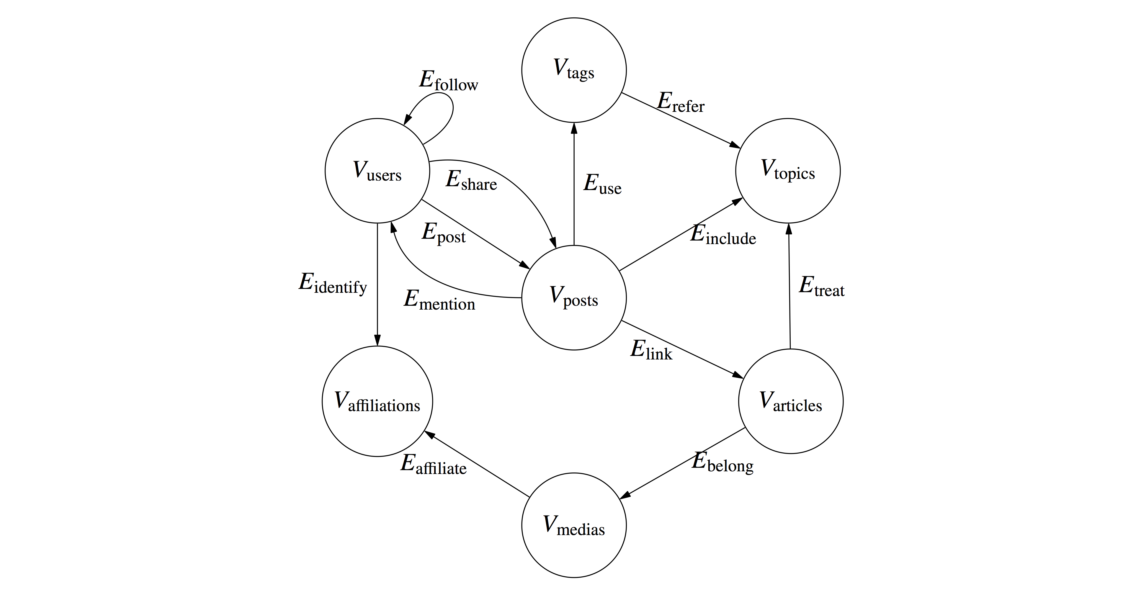
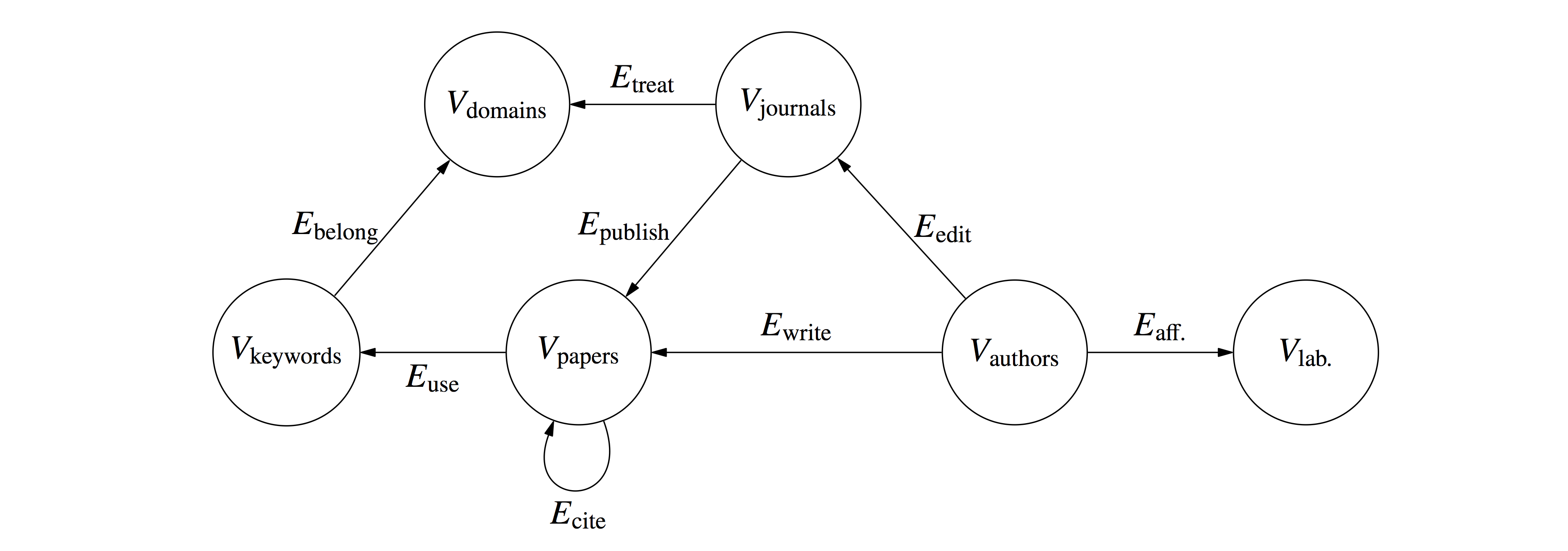
In short: HINPy is a python workbench for Heterogeneous Information Networks (graphs with colored nodes and edges) suited for the analysis of Recommender Systems (accuracy, diversity, similarity), and network representation in other domains (e.g, ecology, scientometrics, social network analysis).

HINPy is a framework that provides a flexible ontology to topological data (entities of different type connected/related by different relations), and allows for the extraction of metrical (similarities, distances), hilbertian (embedding in spaces with relative order), and bayesian (empirical distributions and apportionments) structures.

It also provides [experimental] functionalities to perform recommendations using classic Recommender Systems, and evaluate recommendations with classic diversity metrics.

Also experimental is the extraction of timeseries of apportionments and aggregations such as diversity measures.

Please cite us. Most definitions and computations are taken from:

Ramaciotti Morales, P., Lamarche-Perrin, R., Fournier-S'Niehotta, R., Poulain, R., Tabourier, L. and Tarissan, F., 2021. Measuring Diversity in Heterogeneous Information Networks. Theoretical Computer Science.

Installation

pip install hinpy

Quickstart

Syntax

You can name related entities in lines in a CSV file as:

relation_name,group_of_entity1,name_of_entity1,group_of_entity2,name_of_entity2,some_value,timestamp.

Values (some_value) and timestamps are optional (in case you want to do some filtering or timeseries). In a Recommender Systems setting, for example, you can name your entities and relations as:

has_chosen,users,user1,items,item1,5.0,1990
has_chosen,users,user1,items,item2,3.0,1991
...
was_recommended,user1,items,item4,,
...
is_of_type,items,i1,type,t1,,
...

if you want to declared users that chose/ranked some items (e.g., films) at some time, and items that belong to categories (e.g., genres).

You can then load your CSV (without header nor index):

import hinpy 

hin = hinpy.HIN(filename=path_to_your_csv_file)

A simple example

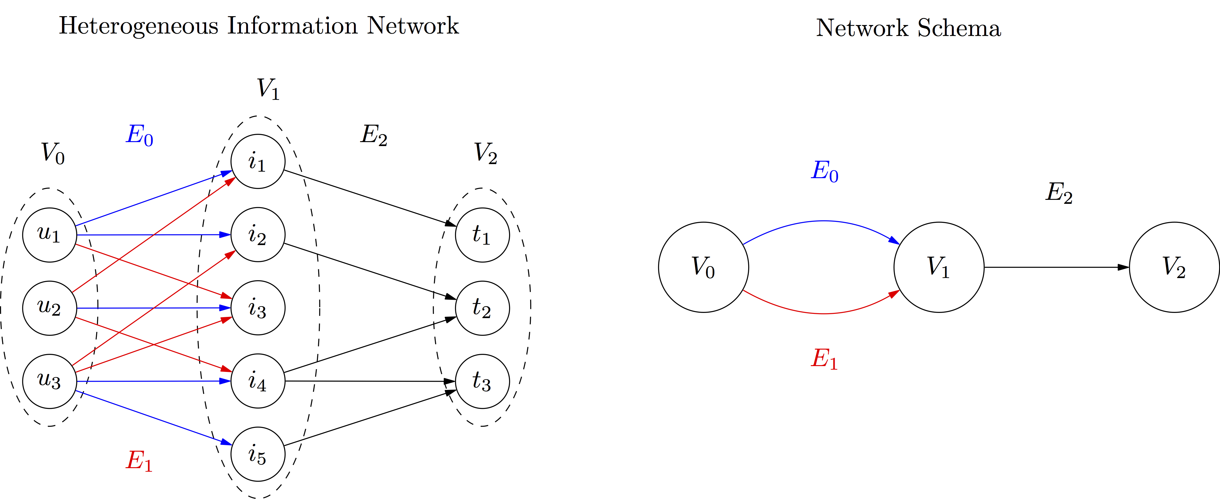
Let us consider entities organized in three object groups, connected with edges organized in three link groups:

The corresponfing file (available in datasets as simple_example.csv) would like something like this:

E0,V0,u1,V1,i1,,
E0,V0,u1,V1,i2,,
E0,V0,u2,V1,i3,,
E0,V0,u3,V1,i4,,
E0,V0,u3,V1,i5,,
E1,V0,u1,V1,i3,,
E1,V0,u2,V1,i1,,
E1,V0,u2,V1,i4,,
E1,V0,u3,V1,i2,,
E1,V0,u3,V1,i3,,
E2,V1,i1,V2,t1,,
E2,V1,i2,V2,t2,,
E2,V1,i4,V2,t2,,
E2,V1,i4,V2,t3,,
E2,V1,i5,V2,t3,,

First, load the file:

import hinpy
hin = hinpy.HIN(filename='simple_example.csv')

Say for example that E0 contains past choices of users in V0 of items in V1, and that item can be associated with categories or types in V2. If E1 contains recommendations made to users, we can measure

-- the mean type diversity of items chosen (E0) by users:

hin.mean_diversity(['E0','E2'],alpha=2.0) # Herfindahl Diversity (alpha=2)
>>> 1.8

-- for comparison, the mean type diversity of items recommended (E1) to users:

hin.mean_diversity(['E1','E2'],alpha=2.0)
>>> 1.8333333333333333

-- which might be also compared with the collective type diversity of items chosen by users:

hin.collective_diversity(['E0','E2'],alpha=2.0)
>>> 2.909090909090909

One can also measure apportionments along paths in the network schema (meta paths). For example:

hin.proportional_abundance(['E0','E2'])
>>> array([0.375, 0.375, 0.25 ])

To see what probability corresponds to which entities you can check to dictionnary of the object group where your path ends (E2), V2:

hin.GetObjectGroupPositionDic('V2')
>>> {'t3': 0, 't2': 1, 't1': 2}

or the other way around:

hin.GetObjectGroupObjectDic('V2')
>>> {0: 't3', 1: 't2', 2: 't1'}

So, in this case, 25% chances of ending in t1, 37.5% for t2 and t3.

You can compute transpose (inverse) meta paths to include in computations

hin = hinpy.HIN(filename='simple_example.csv',inverse_relations=True)

and then used them apportionments and computations (it automatically add the prefix inverse_):

hin.proportional_abundance(['inverse_E2','inverse_E0'])
>>> array([0. , 0.5, 0.5])

If you want to use a different diversity measures (different from True Diversity, which are those used by default, check the article), you can do as you like. Let's use Gini, or Herfindahl-Hirschmann Index (HHI):

pa = hin.proportional_abundance(['E0','E2']) # this was [0.375, 0.375, 0.25 ]
hinpy.diversity.GiniIndex(pa)
>>> 0.3333333333333333
hinpy.diversity.HHI(pa) # Herfindahl-Hirschmann Index
>>> 0.34375

Note that 0.34375 is the reciprocal of the collective E0-E2 Herfindahl (alpha=2) diversity. HHI measures concentration, the reciprocal of diversity.

Once you have a distribution, you do whatever you want with it.

A second example

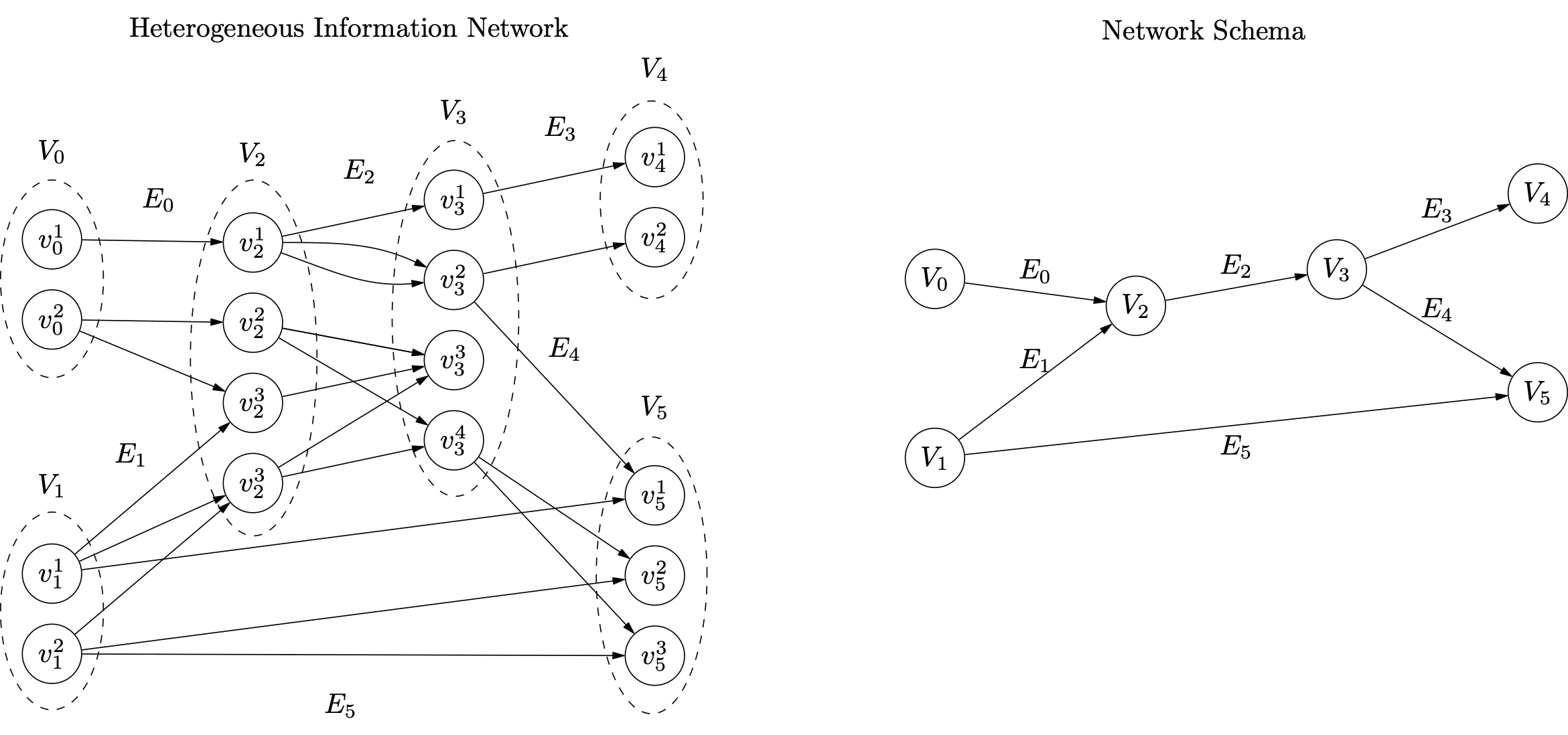
Let us consider now a more complex example.

The file for this example is available in datasets as example.csv:

E0,V0,v01,V2,v21,,
E0,V0,v02,V2,v22,,
E0,V0,v02,V2,v23,,
E1,V1,v11,V2,v23,,
E1,V1,v11,V2,v24,,
E1,V1,v12,V2,v24,,
E2,V2,v21,V3,v31,,
E2,V2,v21,V3,v32,,
E2,V2,v21,V3,v32,,
E2,V2,v22,V3,v33,,
E2,V2,v22,V3,v34,,
E2,V2,v23,V3,v33,,
E2,V2,v24,V3,v33,,
E2,V2,v24,V3,v34,,
E3,V3,v31,V4,v41,,
E3,V3,v32,V4,v42,,
E4,V3,v32,V5,v51,,
E4,V3,v34,V5,v52,,
E4,V3,v34,V5,v53,,
E5,V1,v11,V5,v51,,
E5,V1,v12,V5,v52,,
E5,V1,v12,V5,v53,,

Let us load the file as before:

hin = hinpy.HIN('example.csv',inverse_relations=True)

We can list all the link groups recognized in the input file:

hin.GetLinkGroupsNames()
>>> ['E0', 'E1', 'E2', 'E3', 'E4', 'E5', 'inverse_E0', 'inverse_E1', 'inverse_E2', 'inverse_E3', 'inverse_E4', 'inverse_E5']

You can compute the apportionments (also called proportional abundances), which are probability mass functions resulting from random walks along meta-paths. You can compute the "collective" proportional abundance, starting randomly in an object group

hin.proportional_abundance(path=['E0','E2','E4'])
>>> array([0.16666667, 0.66666667, 0.16666667])

To see the objects to which these probabilities correspond, you have to check

hin.GetObjectGroup('V5').objects_ids
>>> {'v52': 0, 'v51': 1, 'v53': 2}

You can also compute the "individual" proportional abundances, starting in a single object in an objects group

hin.proportional_abundances(path=['E0','E2','E4'])
matrix([[0. , 1. , 0. ],[0.5, 0. , 0.5]])

Using these proportional abundances, you can compute their diversities, as you would with other probability mass functions.

You can compute diversities in arbitrarily longe meta paths:

hin.collective_diversity(['E0','E2','E4'],alpha=1)
>>> 2.3811015779522995

Using inverse relations you can also compose arbitrarily complex meta paths:

hin.collective_diversity(['E0','E2','inverse_E2','E2','E4','inverse_E5'],alpha=1)
>>> 1.9796263300525183

Value propagation/aggregation along meta paths

Since we can produce the proportional abundance of any group of nodes in any other group of nodes following a meta path, we can also use those proportions in the proportional abundance to compute means of values.

The key ingredients are: 1) a dictionary for the values of the node groups whose values you want to aggregate, and 2) a meta path that starts in the node groups that will inherit the values and ends in the node group from where values are to be inherited. The same procedure can be used with any meta path. For example:

V5_values = {'v51':-2,'v52':5,'v53':1}
hin.path_value_aggregation(V5_values, path = ['E0','E2','E4'])
>>> {'v01': -2.0, 'v02': 3.0}

If a node cannot inherit values from a meta path because no set of edges in it link to a target node, the resulting value will be NaN:

hin.path_value_aggregation(V5_values, path = ['E4']) 
>>> {'v31': nan, 'v32': -2.0, 'v34': 3.0, 'v33': nan}

Inverse link groups can be used to estimate score when entities of two groups are related to entities of a third group. Let's say that nodes in V0 have some associated value,

V0_values = {'v01':1,'v02':-1}

and that you want to propagate that value to nodes in V1 using common relation with nodes in V0:

hin.path_value_aggregation(V0_values, path = ['E1','inverse_E0'])
>>> {'v12': nan, 'v11': -1.0}

Time series

If you included information in the timestamp column, you can create new groups of edges (link groups) base on time windows. This allows you to create time series. For the time being this is a bit cumbersome.

Let us take the example file movielens100k_hin.csv (found in the datasets folder). This is a classic dataset in Recommender Systems, containing information on people rating films between 1997 and 1998.

import hinpy
import numpy
import calendar

hin = hinpy.classes.HIN(filename='movielens100k_hin.csv')

Let us check the link groups it contains:

hin.GetLinkGroupsNames()
>>> ['is_of_type','was_released','rates','has_occupation','has_age','has_gender','is_located']

... and its object groups:

hin.GetObjectGroupsNames()
>>> ['age','occupation','genre','zip_code','user','movie','gender','release']

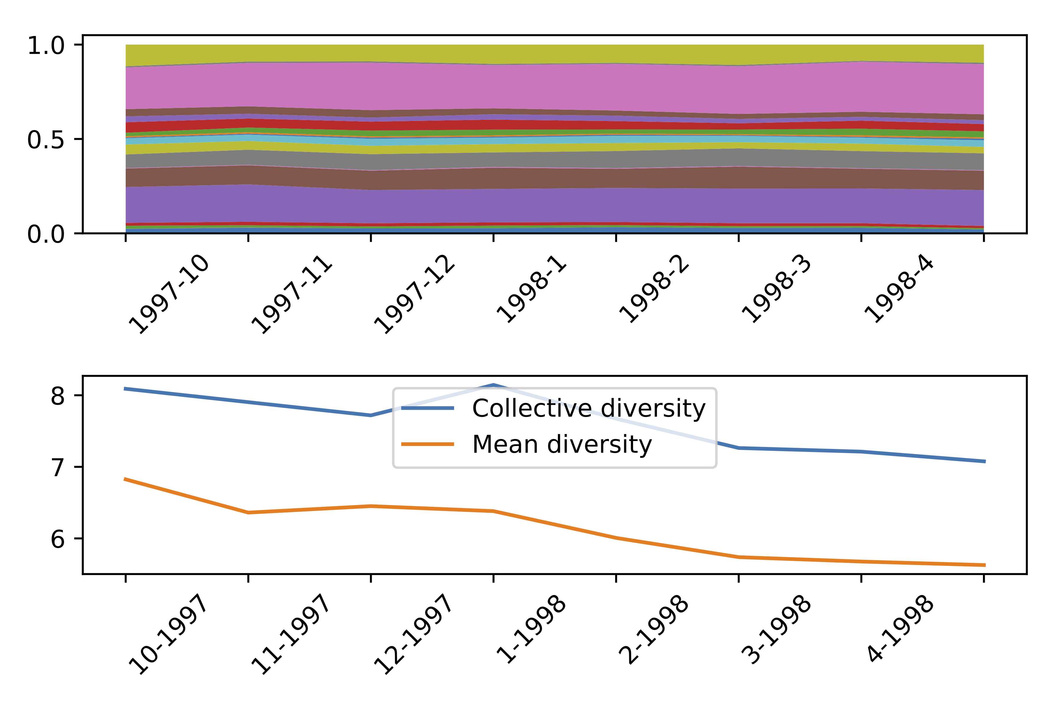
A lot of information. Let us focus on users that rate movies that have a genre. The link group called rates, has timestamps. In the next piece of code we iterate through months to make a temporal series of genre diversity of movies rated by users:

months =  [(9,1997),(10,1997),(11,1997),(12,1997),(1,1998),(2,1998),(3,1998),(4,1998)]
N_genres = hin.GetObjectGroup('genre').size # there are 19 film genres

collective_diversity = [] # <- time series
mean_diversity = [] # <- time series
collective_pa = np.zeros((N_genres,len(months))) # <- apportionment time series

for i,(month,year) in enumerate(months):
    # we give first and last days to define a timewindow
    first_day = '%d-%d-%d'%(year,month,1)
    last_day  = '%d-%d-%d'%(year,month,calendar.monthrange(year,month)[1])
    window = {'min':first_day,'max':last_day,}
    # then create a new link group using "rates"
    hin.CreateLinkGroup(linkgroup='rates',name='monthly_activity',datetimes=window)
    # then we compute proportional abundance, and diversities
    collective_diversity.append(hin.collective_diversity(['monthly_activity','is_of_type'],alpha=2.0))
    mean_diversity.append(hin.mean_diversity(['monthly_activity','is_of_type'],alpha=2.0))
    collective_pa[:,i] = hin.proportional_abundance(['monthly_activity','is_of_type'])
    # and we delete the link group we created for this month
    hin.DeleteLinkGroup('monthly_activity')
    
import matplotlib.pyplot as plt
fig, axs = plt.subplots(2, 1)
axs[0].stackplot(np.arange(len(months)),collective_pa,baseline='zero')
axs[0].set_xticklabels(['%d-%d'%(y,m) for m,y in months],rotation = 45, ha="left")
axs[1].plot(np.arange(len(months)),collective_diversity)
axs[1].plot(np.arange(len(months)),mean_diversity)
axs[1].legend(['Collective diversity','Mean diversity'])
axs[1].set_xticklabels(['%d-%d'%(y,m) for y,m in months],rotation = 45, ha="left")

Producing and evaluating recommendations

Upcoming section. You can take a peek in the examples folder.

Applications in other domains

This framework might be useful in many domains besides Recommender Systems.

Feel free to use it in social network analysis and computational social sciences

in ecology

in comptetion law and antitrust

or in scientometrics

among many others.