Home
Welcome to the grasshopper wiki!

grasshopper is a front-end for Geant4, which allows the user to define all the aspects of the simulation is a single Geometry Definition Markup Language (GDML) file:particles to be emitted, the materials which the particle will interact with, and the output desired. The input file is then read by the dedicated Geant4 application (in this case: grasshopper), and a simulation is run. This framework significantly simplifies the "learning curve" and the barrier to entry to Geant4, allowing researchers and students alike to quickly set up and run simple simulations.
The tutorial below will teach students at MIT to use the NSE computational facilities to run grasshopper and analyze and interpret its output.
NOTE: the "Basic requirements" and "Settings things up" sections are only for the MIT NSE students who have accounts on nsecsluter.mit.edu. Feel free to skip.
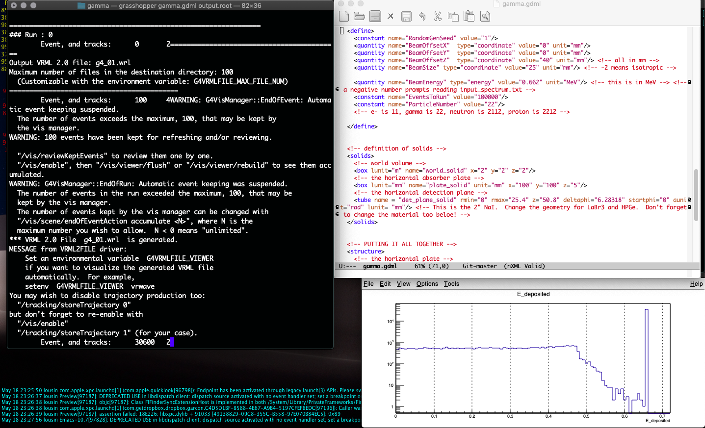
A view of your workspace:
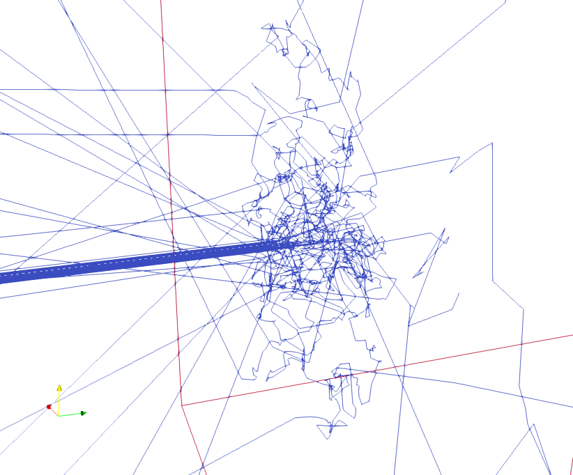
Below -- a visualization of a 1 MeV neutron beam entering a water volume, undergoing thermalization.
(For MIT NSE students only)
- at a minimum you will need to login to nsecluster.mit.edu.
- From a terminal run
ssh -Y [email protected]- OR, which is simpler -- login via nsecluster.mit.edu/jhub/hub/login
- for either option you'll need an account -- ask [email protected] or [email protected]
- the windows users can either use cygwin, PUTTY or some ssh client. Although we strongly recommend that you get ubuntu going via WSL(for Windows 10/11) -- once there you can get ssh via
sudo apt install ssh - for additional (good, detailed, recommended) instructions, please see here and here.
- From a terminal run
- Install paraview on your laptop. This will allow you to inspect the visualization VRML files generated by grasshopper (one picture's worth a thousand words, a 3D rendering is worth a billion).
- you will also need to have some basic ability of working in linux environment. See here for a brief tutorial.
(For MIT NSE students only)
Once you log in into your account on nsecluster, you need to copy over a few files, directories, and run some scripts.
> cd #this is a comment. A cd by itself drops you into your home directory> cp .bashrc .bashrc_save && cp ~aregjan/.bashrc . #this is a comment. .bashrc is your configuration file. Note that this will overwrite your own .bashrc> cp ~aregjan/.nanorc .> cp -r ~aregjan/.nano . #these are for enabling syntax highlighting in nano, quite useful> source .bashrc #execute the settings> cp -r ~aregjan/github.com/grasshopper/exec/Examples . #this is your work directory. Go ahead, look inside.
Now you are ready to run. But can you analyze the output? In class we will use these two jupyter notebooks to read in the grasshopper output, histogram it, and make sense of it all.
- Please download the following notebook1
- Optional, but strongly recommended: get also the following notebook which uses PyROOT for data analysis.
- Please note that for PyROOT to work you need to install it via conda:
> conda install pyroot
If you do
>ls Examples
you will see three directories, named after the three experiments in your class. Let's go into one of them:
> cd Examples/beta
> ls beta.gdml beta_lite.gdml
In this tutorial we'll focus on beta_lite.gdml, a simple simulation of shooting a pencil beam of 1MeV electrons onto your detector at a distance of 20cm away. Let's look inside beta_lite.gdml, to understand the general structure of the input. In general, the file is heavily commented, and as such is quite self-explanatory. There are six sections:
-
MATERIALS This is where some of the materials are defined. Note that Geant4 has many, many pre-defined materials, significantly simplifying setup. The listing of these can be found in
~/22.09/documentation/materials_listing.pdf. - THE OUTPUT This is where you specify what kind of output you want. Most of the time we won't change these.
- CUTS This section defines a number of variables which can be used to improve the computational efficiency. Changing these haphazardly can produce incorrect results, however. Again, this should not be changed much.
- OUTPUT FILTERS This is where you define what type of information you want to keep in the simulation output. For the alpha and beta simulation, where you only care for the flux of the particles at the entrance of your detector, simply set SaveSurfaceHitTrack to 1, and everything else to 0. For gamma spectroscopy, where you need to determine the energy deposition in the detector, set SaveEdepositedTotalEntry to 1 and everything else to 0.
- THE BEAM This is where we define the particle type we want to run. BeamOffsetX/Y/Z define the starting point of the particle. Beam Energy of -1 will cause the simulation to read in and sample the energy from input_spectrum.txt file, which defines the energy distribution of the particles. ParticleNumber defines the actual particle! The scheme for particle types is defined by the Particle Data Group, and include a vast set of particles and nuclei. For us some of the most useful particles are e^-, gamma, neutrons, protons, and alphas, and their PID's are 11, 22, 2112, 2212, and 1000020040, respectively.
-
GEOMETRIES This section follows the general Geant4 scheme of creating a shape/geometry (
<solids>), filling it with materials and positioning it (<structure>). For the later stage on needs to fill the solid with materials (<volume>) and position it (<physvol>).
In order for your code to produce an output you need to have one or more detector volumes. grasshopper identifies a detector as any volume whose physical placement is named det_phys#, where # is the desired detector number. The code will parse the name and extract the detector number, which will show up in the output. For SaveSurfateHit mode only the first detector hit by the track will be recorded.
The simulation described in beta_lite.gdml is that of a 2 MeV electron beam traversing a 0.25mm Al absorber, and then impinging on the detector further downstream.
So let's do it!
>cd ~/Examples/beta
>grasshopper beta_lite.gdml test
Assuming you set everything up right, you'll get lots of output, indicating that the simulation is running.
Once it's over exit Torque by typing exit -- this will drop you back to the head node.
At the completion of the run, you'll see three new files:
-
test.root...this is the output in ROOT format assuming you enabled it (default: disabled), which can be loaded into root and the results of the simulation analyzed. -
test.dat...this is simply the ascii version of the above, which you can load into your tool of choice (python, MATLAB, gnuplot, R). Because we set BriefOutputOn to 1 in the GDML file, beta_lite.dat will contain a very minimal output -- just the energy (either incident, or deposited, depending on your choice of output filters) in MeV, the EventID, the particle name and the process which created it. Optional: if you want to access the full trove of output from the simulation, then simply set BriefOutputOn to zero. The structure of the rich output can be found in README.md. -
g4_00.wrlthis contains the visualization of the simulation. You should copy this over to your laptop (along with the other files), and load it into paraview for a visual inspection. Note: with every new run the index ofg4_00.wrlgets incremented, to prevent overwriting.
For this particular simulation, you can see the energy distribution of the electrons hitting the detector in the plot below (from ROOT):

Also, here is the view of the g4_00.wrl in paraview:

Now that you got the simulation running, feel free to play with beta_lite.gdml and modify the absorber thickness. Load the output into your analysis tool of choice and re-plot the energy distribution as above. What happens to the counts and the average energy as you increase the absorber thickness?
There are a few documents describing the various inputs into the GDML file. These are all located in ~/22.09/documentation directory. The files are, in order of importance:
- materials_listing.pdf The Geant4 input allows you to define your own materials from "scratch" from individual isotopes. You can define your own elements, and then produce materials from those elements. The header of the GDML file contains a few examples, for reference. However, the GDML also has a (fairly large) set of pre-defined materials. materials_listing.pdf contains the list of all those pre-defined materials and is quite self-explanatory.
- GDMLmanual.pdf As the name implies, this is the manual for the GDML input to Geant4.
- montecarlorpp.pdf This file lists all the PID numbers, as defined by the LLNL Particle Data Group. This is useful only if you want to go off the beaten path and simulate particles other than alpha, beta, gamma, or neutrons (something you are very much encouraged to do!).
While grasshopper tries to have a systematic way of defining geometries, run conditions, etc., over time a number of built-in "hacks" (primarily for rarely used conditions) have been introduced - as a way of keeping the gdml input as simple as possible. These are likely to go away in the next major versions of the code and be replaced with dedicated flags. Below is a comprehensive list:
- Beam Energy If beam energy is set to a negative number then the code automatically reads in the input_spectrum.txt file, which describes the distribution from which the energy will be sampled. Specifically, a value of -2 MeV (recommended) will results in an interpolative sampling based on the input from input_spectrum.txt. -3 on the other hand will treat the entries in input_spectrum.txt as single energies, i.e. as in the case of a combination of isotopic sources.
-
Beam Size If the beam size is negative then one of the following happens:
- if(beam_size==-1): the beam is described as a narrow fan beam. The only way to change this is by modifying the code in PrimaryGeneratorAction.cc
- if(beam_size==-2): isotropic beam
- if(beam_size==-3): omnidirectional beam
- else if(beam_size<0): i.e. any negative number other than -1, -2, or -3 -- the beam spot size is abs(beam_size), however the output is isotropic. Furthermore, if beam_width.txt is found, then the code reads its content (a single number) which defines the width of the source. This mode of operation could be used to describe a decaying source of gas, e.g. tritium gas. For a flat isotropic source (e.g. a typical alpha source) simply set beam_size=-(source radius).
Ok, time to get the grasshopper jumping! You are tasked with simulating the passage of the alpha particles through air. We want to know the energy distributions of 5.5 MeV alphas as they traverse exactly 42 mm of air. Use beta_lite.gdml as a starting point. You need to perform the following modifications:
- switch from e- to alphas
- set the detector at 42 mm
- it helps reducing the number of counts to run to 10 000 (unless you are willing to run for long time!)
- and most importantly - get rid of the Al plate. There are two ways of doing this
- actually get rid of it in the physical volume placement (delete the lines)
- or, simply replace its material with
G4_AIR.
We want you to give us the following information:
- How many alphas reach the detector plane
- What is their energy? St. deviation?
- plot their energy distribution / spectrum
- use ASTAR to determine the ionization energy loss for 5.5 MeV alphas in 42 mm of dry air. How does this compare to the simulation results?
Grasshoppers hate bugs. The code has been tested fairly well, however there are probably still some bugs in it. If you run against a strange behavior, please prepare a brief report with the following information
- the platform you are running it on
- the gdml file (attach it)
- a description of the symptoms, along with the relevant part of the screen output
and email it all to mailto:[email protected].