MedicalCostPrediction 🧠

Machine learning model to predict the medical cost of pacients using Python and multiple linear regression.

Data cleaning 📊

The original dataset has six independent variables: age, sex, bmi, children, smoker, region, and one output: charges.

age	sex	bmi	children	smoker	region	charges
19	female	27.9	0	yes	southwest	16884.924
18	male	33.77	1	no	southeast	1725.5523
28	male	33	3	no	southeast	4449.462
33	male	22.705	0	no	northwest	21984.47061

The values for sex, children, smoker and region are dummy variables, so we need to convert them. For smoker label encoding should be enough, but for the other values one-hot encoding is better, because nothing ensures that one particular sex, children or region will have higher costs.

age	bmi	smoker	charges	children_0	children_1	children_2	children_3	children_4	children_5	sex_female	sex_male	region_northeast	region_northwest	region_southeast	region_southwest
19	27.9	1	16884.92	1	0	0	0	0	0	1	0	0	0	0	1
18	33.77	0	1725.55	0	1	0	0	0	0	0	1	0	0	1	0
28	33.0	0	4449.46	0	0	0	1	0	0	0	1	0	0	1	0
33	22.705	0	21984.47	1	0	0	0	0	0	0	1	0	1	0	0

After this, since we will be using gradient descent to perform our training, the data normalization should be done, to avoid extra cost in the training algorithm.

age	bmi	smoker	charges	children_0	children_1	children_2	children_3	children_4	children_5	sex_female	sex_male	region_northeast	region_northwest	region_southeast	region_southwest
0.021739130434782608	0.3212267958030669	1.0	0.25161073135599604	1.0	0.0	0.0	0.0	0.0	0.0	1.0	0.0	0.0	0.0	0.0	1.0
0.0	0.479149852031208	0.0	0.009635975671268423	0.0	1.0	0.0	0.0	0.0	0.0	0.0	1.0	0.0	0.0	1.0	0.0
0.21739130434782608	0.4584342211460855	0.0	0.053115187324337544	0.0	0.0	0.0	1.0	0.0	0.0	0.0	1.0	0.0	0.0	1.0	0.0
0.32608695652173914	0.18146354587032545	0.0	0.3330100484352713	1.0	0.0	0.0	0.0	0.0	0.0	0.0	1.0	0.0	1.0	0.0	0.0

And know the data is ready to be used, it just needs to be separated between the training and testing dataset, what can be done using sklearn function train_test_split.

Model training 🔄

The cost function chosen for this model was the Mean Squared Error, which can calculate the divergence between the hypothesis and the actual cost output.

For every iteration, the cost function is calculated and should be minimized ultil convergence, a state where almost nothing changes anymore. To minimize the function, the model uses the derivative of gradient descent for each theta parameter, and update all of them simultaneously.

This way, if everything is working and a good learning rate α is chosen, the Mean Squared Error should decrease in every iteration, improving the model precision.

Model testing 📚

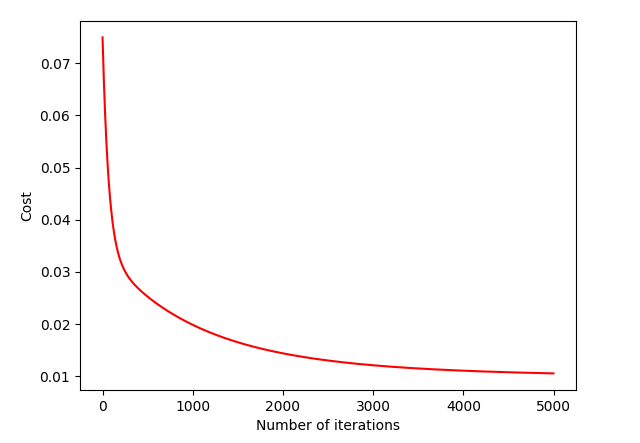
The test of the model was made using the dataset that was initially separated from the training set. For the test, the hypothesis of each sample was calculated, based on the theta values generated from training. Then, the algorithm calculates R-squared to get the overall model precision.

Results

Training the algorithm with iters = 10000 and α = 0.003:

And here are some examples of the hypothesis of the model and the real costs

hypothesis	y
0.1479535293752109	0.12726868742074837
0.09149105409187717	0.06624749236055866
0.5627710769272539	0.45027547321119593
0.13548529518828206	0.13056996042686375

Technologies 💻

Build with:

• Python
• pandas
• NumPy
• matplotlib
• scikit-learn

Author 🧙

• viniciuslazzari