isosurface.scad
Metaballs (also known as "blobby objects"), are bounded and closed organic surfaces that smoothly blend together. Metaballs are a specific kind of isosurface.
An isosurface, or implicit surface, is a three-dimensional surface representing all points of a constant value (e.g. pressure, temperature, electric potential, density) in a 3D volume. It's the 3D version of a 2D contour; in fact, any 2D cross-section of an isosurface is a 2D contour.
For computer-aided design, isosurfaces of abstract functions can generate complex curved surfaces and organic shapes. For example, spherical metaballs can be formulated using a set of point centers that define the metaballs locations. For metaballs, a function is defined for all points in a 3D volume based on the distance from any point to the centers of each metaball. The combined contributions from all the metaballs results in a function that varies in a complicated way throughout the volume. When two metaballs are far apart, they appear simply as spheres, but when they are close together they enlarge, reach toward each other, and meld together in a smooth fashion. The resulting metaball model appears as smoothly blended blobby shapes. The implementation below provides metaballs of a variety of types including spheres, cuboids, and cylinders (cones), with optional parameters to adjust the influence of one metaball on others, and the cutoff distance where the metaball's influence stops.
In general, an isosurface can be defined using any function of three variables
Some isosurface functions are unbounded, extending infinitely in all directions. A familiar example may be a gryoid, which is often used as a volume infill pattern in fused filament fabrication. The gyroid isosurface is unbounded and periodic in all three dimensions.
This file provides modules and functions to create a VNF using metaballs, or from general isosurfaces.
The point list in the generated VNF structure contains many duplicated points. This is normally not a
problem for rendering the shape, but machine roundoff differences may result in Manifold issuing
warnings when doing the final render, causing rendering to abort if you have enabled the "stop on
first warning" setting. You can prevent this by passing the VNF through vnf_quantize() using a
quantization of 1e-7, or you can pass the VNF structure into vnf_merge_points(), which also
removes the duplicates. Additionally, flat surfaces (often resulting from clipping by the bounding
box) are triangulated at the voxel size resolution, and these can be unified into a single face by
passing the vnf structure to vnf_unify_faces(). These steps can be computationally expensive
and are not normally necessary.
To use, add the following lines to the beginning of your file:
include <BOSL2/std.scad>
include <BOSL2/isosurface.scad>
-
metaballs()– Creates a group of 3D metaballs (smoothly connected blobs). [Geom] [VNF] -
isosurface()– Creates a 3D isosurface (a 3D contour) from a function or array of values. [Geom] [VNF]
Synopsis: Creates a group of 3D metaballs (smoothly connected blobs). [Geom] [VNF]
Topics: Metaballs, Isosurfaces, VNF Generators
See Also: isosurface()
Usage: As a module
- metaballs(spec, bounding_box, voxel_size, [isovalue=], [closed=], [exact_bounds=], [convexity=], [show_stats=], ...) [ATTACHMENTS];
Usage: As a function
- vnf = metaballs(spec, bounding_box, voxel_size, [isovalue=], [closed=], [exact_bounds=], [convexity=], [show_stats=]);
Description:
Metaballs, also known as "blobby objects", can produce smoothly varying blobs and organic forms. You create metaballs by placing metaball objects at different locations. These objects have a basic size and shape when placed in isolation, but if another metaball object is nearby, the two objects interact, growing larger and melding together. The closer the objects are, the more they blend and meld.
The simplest metaball specification is a 1D list of alternating transformation matrices and
metaball functions: [trans0, func0, trans1, func1, ... ]. Each transformation matrix
you supply can be constructed using the usual transformation commands such as up(),
right(), back(), move(), scale(), rot() and so on. You can multiply
the transformations together, similar to how the transformations can be applied
to regular objects in OpenSCAD. For example, to transform an object in regular OpenSCAD you
might write up(5) xrot(25) zrot(45) scale(4). You would provide that transformation
as the transformation matrix up(5) * xrot(25) * zrot(45) * scale(4). You can use
scaling to produce an ellipsoid from a sphere, and you can even use skew() if desired.
When no transformation is needed, give IDENT as the transformation.
The metaballs are evaluated over a bounding box, which can be specified by its
minimum and maximum corners [[xmin,ymin,zmin],[xmax,ymax,zmax]],
or specified as a scalar size of a cube centered on the origin. The contributions from all
metaballs, even those outside the box, are evaluated over the bounding box. This bounding box is
divided into voxels of the specified voxel_size, which can also be a scalar cube or a vector size.
Alternately, voxel_count may be specified to set the voxel size according to the requested
count of voxels in the bounding box.
Smaller voxels produce a finer, smoother result at the expense of execution time. By default, if the
voxel size doesn't exactly divide your specified bounding box, then the bounding box is enlarged to
contain whole voxels, and centered on your requested box. Alternatively, you may set
exact_bounds=true to cause the voxels to adjust in size to fit instead. Either way, if the
bounding box clips a metaball and closed=true (the default), the object is closed at the
intersection surface. Setting closed=false causes the VNF faces to end at the bounding
box, resulting in a non-manifold shape with holes, exposing the inside of the object.
For metaballs with flat surfaces (the ends of mb_cyl(), and mb_cuboid() with squareness=1),
avoid letting any side of the bounding box coincide with one of these flat surfaces, otherwise
unpredictable triangulation around the edge may result.
You can create metaballs in a variety of standard shapes using the predefined functions
listed below. If you wish, you can also create custom metaball shapes using your own functions
(see Examples 20 and 21). For all of the built-in metaballs, three parameters are available to control
the interaction of the metaballs with each other: cutoff, influence, and negative.
The cutoff parameter specifies the distance beyond which the metaball has no interaction
with other balls. When you apply cutoff, a smooth suppression factor begins
decreasing the interaction strength at half the cutoff distance and reduces the interaction to
zero at the cutoff. Note that the smooth decrease may cause the interaction to become negligible
closer than the actual cutoff distance, depending on the voxel size and influence of the
ball. Also, depending on the value of influence, a cutoff that ends in the middle of
another ball can result in strange shapes, as shown in Example 17, with the metaball
interacting on one side of the boundary and not interacting on the other side. If you scale
a ball, the cutoff value is also scaled. The exact way that cutoff is defined
geometrically varies for different ball types; see below for details.
The influence parameter adjusts the strength of the interaction that metaball objects have with
each other. If you increase influence of one metaball from its default of 1, then that metaball
interacts with others at a longer range, and surrounding balls grow bigger. The metaball with larger
influence can also grow bigger because it couples more strongly with other nearby balls, but it
can also remain nearly unchanged while influencing others when isovalue is greater than 1.
Decreasing influence has the reverse effect. Small changes in influence can have a large
effect; for example, setting influence=2 dramatically increases the interactions at longer
distances, and you may want to set the cutoff argument to limit the range influence.
At the other exteme, small influence values can produce ridge-like artifacts or texture on the
model. Example 14 demonstrates this effect. To avoid these artifacts, keep influence above about
0.5 and consider using cutoff instead of using small influence.
The negative parameter, if set to true, creates a negative metaball, which can result in
hollows, dents, or reductions in size of other metaballs.
Negative metaballs are never directly visible; only their effects are visible. The influence
argument may also behave in ways you don't expect with a negative metaball. See Examples 16 and 17.
For complicated metaball assemblies you may wish to repeat a structure in different locations or
otherwise transformed. Nested metaball specifications are supported:
Instead of specifying a transform and function, you specify a transform and then another metaball
specification. For example, you could set finger=[t0,f0,t1,f1,t2,f2] and then set
hand=[u0,finger,u1,finger,...] and then invoke metaballs() with [s0, hand].
In effect, any metaball specification array can be treated as a single metaball in another specification array.
This is a powerful technique that lets you make groups of metaballs that you can use as individual
metaballs in other groups, and can make your code compact and simpler to understand. See Example 23.
The isovalue parameter applies globally to all your metaballs and changes the appearance of your entire metaball object, possibly dramatically. It defaults to 1 and you don't usually need to change it. If you increase the isovalue, then all the objects in your model shrink, causing some melded objects to separate. If you decrease it, each metaball grows and melds more with others.
Built-in metaball functions
Several metaballs are defined for you to use in your models.
All of the built-in metaballs take positional and named parameters that specify the size of the
metaball (such as height or radius). The size arguments are the same as those for the regular objects
of the same type (e.g. a sphere accepts both r for radius and the named parameter d= for
diameter). The size parameters always specify the size of the metaball in isolation with
isovalue=1. The metaballs can grow much bigger than their specified sizes when they interact
with each other. Changing isovalue also changes the sizes of metaballs. They grow bigger than their
specified sizes, even in isolation, if isovalue < 1 and smaller than their specified sizes if
isovalue > 1.
The built-in metaball functions are listed below. As usual, arguments without a trailing = can be used positionally; arguments with a trailing = must be used as named arguments.
-
mb_sphere(r|d=)— spherical metaball, with radius r or diameter d. You can create an ellipsoid usingscale()as the last transformation entry of the metaballspecarray. -
mb_cuboid(size, [squareness=])— cuboid metaball with rounded edges and corners. The corner sharpness is controlled by thesquarenessparameter ranging from 0 (spherical) to 1 (cubical), and defaults to 0.5. Thesizeparameter specifies the dimensions of the cuboid that circumscribes the rounded shape, which is tangent to the center of each cube face.sizemay be a scalar or a vector, as incuboid(). Except whensquareness=1, the faces are always a little bit curved. -
mb_cyl(h|l|height|length, [r|d=], [r1=|d1=], [r2=|d2=], [rounding=])— vertical cylinder or cone metaball with the same dimensional arguments ascyl(). At least one of the radius or diameter arguments is required. Theroundingargument defaults to 0 (sharp edge) if not specified. Only one rounding value is allowed: the rounding is the same at both ends. For a fully rounded cylindrical shape, consider usingmb_capsule()ormb_disk(), which are less flexible but have faster execution times. -
mb_disk(h|l|height|length, r|d=)— rounded disk with flat ends. The diameter specifies the total diameter of the shape including the rounded sides, and must be greater than its height. -
mb_capsule(h|l|height|length, [r|d=]— vertical cylinder or cone with rounded caps, using the same dimensional arguments ascyl(). The object resembles a convex hull of two spheres. The height or length specifies the distance between the spherical centers of the ends. -
mb_connector(p1, p2, [r|d=])— a connecting rod of radiusror diameterdwith hemispherical caps (likemb_capsule()), but specified to connect pointp1to pointp2(wherep1andp2must be different 3D coordinates). As withmb_capsule(), the object resembles a convex hull of two spheres. The pointsp1andp2are at the centers of the two round caps. The connectors themselves are still influenced by other metaballs, but it may be undesirable to have them influence others, or each other. If two connectors are connected, the joint may appear swollen unlessinfluenceorcutoffis reduced. Reducingcutoffis preferable if feasible, because reducinginfluencecan produce interpolation artifacts. -
mb_torus([r_maj|d_maj=], [r_min|d_min=], [or=|od=], [ir=|id=])— torus metaball oriented perpendicular to the z axis. You can specify the torus dimensions using the same arguments astorus(); that is, major radius (or diameter) withr_majord_maj, and minor radius and diameter usingr_minord_min. Alternatively you can give the inner radius or diameter withiroridand the outer radius or diameter withororod. You must provide a combination of inputs that completely specifies the torus. Ifcutoffis applied, it is measured from the circle represented byr_min=0. -
mb_octahedron(size, [squareness=])— octahedron metaball with rounded edges and corners. The corner sharpness is controlled by thesquarenessparameter ranging from 0 (spherical) to 1 (sharp), and defaults to 0.5. Thesizeparameter specifies the tip-to-tip distance of the octahedron that circumscribes the rounded shape, which is tangent to the center of each octahedron face.sizemay be a scalar or a vector, as inoctahedron(). Atsquareness=0, the shape reduces to a sphere curcumscribed by the octahedron. Except whensquareness=1, the faces are always curved.
In addition to the dimensional arguments described above, all of the built-in functions accept the following named arguments:
-
cutoff— positive value giving the distance beyond which the metaball does not interact with other balls. Cutoff is measured from the object's center. Default: INF -
influence— a positive number specifying the strength of interaction this ball has with other balls. Default: 1 -
negative— when true, creates a negative metaball. Default: false
Metaball functions and user defined functions
You can construct complicated metaball models using only the built-in metaball functions above. However, you can create your own custom metaballs if desired.
When multiple metaballs are in a model, their functions are summed and compared to the isovalue to
determine the final shape of the metaball object.
Each metaball is defined as a function of a 3-vector that gives the value of the metaball function
for that point in space. As is common in metaball implementations, we define the built-in metaballs using an
inverse relationship where the metaball functions fall off as
To adjust interaction strength, the influence parameter applies an exponent, so if influence=a
then the decay becomes
You can pass a custom function as a function literal
that takes a single argument (a 3-vector) and returns a single numerical value.
Generally, the function should return a scalar value that drops below the isovalue somewhere within your
bounding box. If you want your custom metaball function to behave similar to to the built-in functions,
the return value should fall off with distance as influence and cutoff.
Voxel size and bounding box
The size of the voxels and size of the bounding box affects the run time, which can be long.
A voxel size of 1 with a bounding box volume of 200×200×200 may be slow because it requires the
calculation and storage of 8,000,000 function values, and more processing and memory to generate
the triangulated mesh. On the other hand, a voxel size of 5 over a 100×100×100 bounding box
requires only 8,000 function values and a modest computation time. A good rule is to keep the number
of voxels below 10,000 for preview, and adjust the voxel size smaller for final rendering. If you don't
specify either voxel_size or voxel_count, then a default count of 10,000 voxels is used,
which should be reasonable for initial preview. Because a bounding
box that is too large wastes time computing function values that are not needed, you can also set the
parameter show_stats=true to get the actual bounds of the voxels intersected by the surface. With this
information, you may be able to decrease run time, or keep the same run time but increase the resolution.
Duplicated vertices
The point list in the generated VNF structure contains many duplicated points. This is normally not a
problem for rendering the shape, but machine roundoff differences may result in Manifold issuing
warnings when doing the final render, causing rendering to abort if you have enabled the "stop on
first warning" setting. You can prevent this by passing the VNF through vnf_quantize() using a
quantization of 1e-7, or you can pass the VNF structure into vnf_merge_points(), which also
removes the duplicates. Additionally, flat surfaces (often resulting from clipping by the bounding
box) are triangulated at the voxel size resolution, and these can be unified into a single face by
passing the vnf structure to vnf_unify_faces(). These steps can be computationally expensive
and are not normally necessary.
Arguments:
| By Position | What it does |
|---|---|
spec |
Metaball specification in the form [trans0, spec0, trans1, spec1, ...], with alternating transformation matrices and metaball specs, where spec0, spec1, etc. can be a metaball function or another metaball specification. See above for more details, and see Example 23 for a demonstration. |
bounding_box |
The volume in which to perform computations, expressed as a scalar size of a cube centered on the origin, or a pair of 3D points [[xmin,ymin,zmin], [xmax,ymax,zmax]] specifying the minimum and maximum box corner coordinates. Unless you set exact_bounds=true, the bounding box size may be enlarged to fit whole voxels. |
voxel_size |
Size of the voxels used to sample the bounding box volume, can be a scalar or 3-vector, or omitted if voxel_count is set. You may get a non-cubical voxels of a slightly different size than requested if exact_bounds=true. |
| By Name | What it does |
|---|---|
voxel_count |
Approximate number of voxels in the bounding box. If exact_bounds=true then the voxels may not be cubes. Use with show_stats=true to see the corresponding voxel size. Default: 10000 (if voxel_size not set) |
isovalue |
A scalar value specifying the isosurface value (threshold value) of the metaballs. At the default value of 1.0, the internal metaball functions are designd so the size arguments correspond to the size parameter (such as radius) of the metaball, when rendered in isolation with no other metaballs. Default: 1.0 |
closed |
When true, close the surface if it intersects the bounding box by adding a closing face. When false, do not add a closing face, possibly producing non-manfold metaballs with holes where the bounding box intersects them. Default: true |
exact_bounds |
When true, shrinks voxels as needed to fit whole voxels inside the requested bounding box. When false, enlarges bounding_box as needed to fit whole voxels of voxel_size, and centers the new bounding box over the requested box. Default: false |
show_stats |
If true, display statistics about the metaball isosurface in the console window. Besides the number of voxels that the surface passes through, and the number of triangles making up the surface, this is useful for getting information about a possibly smaller bounding box to improve speed for subsequent renders. Enabling this parameter has a small speed penalty. Default: false |
convexity |
(Module only) Maximum number of times a line could intersect a wall of the shape. Affects preview only. Default: 6 |
show_box |
(Module only) display the requested bounding box as transparent. This box may appear slightly inside the bounds of the figure if the actual bounding box had to be expanded to accommodate whole voxels. Default: false |
cp |
(Module only) Center point for determining intersection anchors or centering the shape. Determines the base of the anchor vector. Can be "centroid", "mean", "box" or a 3D point. Default: "centroid" |
anchor |
(Module only) Translate so anchor point is at origin (0,0,0). See anchor. Default: "origin"
|
spin |
(Module only) Rotate this many degrees around the Z axis after anchor. See spin. Default: 0
|
orient |
(Module only) Vector to rotate top toward, after spin. See orient. Default: UP
|
atype |
(Module only) Select "hull" or "intersect" anchor type. Default: "hull" |
Anchor Types:
| Anchor Type | What it is |
|---|---|
| "hull" | Anchors to the virtual convex hull of the shape. |
| "intersect" | Anchors to the surface of the shape. |
Named Anchors:
| Anchor Name | Position |
|---|---|
| "origin" | Anchor at the origin, oriented UP. |
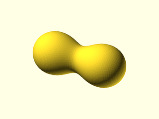
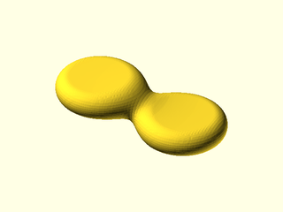
Example 1: Two spheres interacting.
include <BOSL2/std.scad>
include <BOSL2/isosurface.scad>
spec = [
    left(9), mb_sphere(5),
    right(9), mb_sphere(5)
];
metaballs(spec, voxel_size=0.5,
    bounding_box=[[-16,-7,-7], [16,7,7]]);
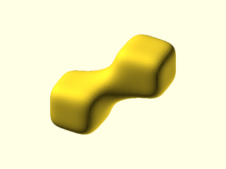
Example 2: Two rounded cuboids interacting.
include <BOSL2/std.scad>
include <BOSL2/isosurface.scad>
spec = [
    move([-8,-5,-5]), mb_cuboid(10),
    move([8,5,5]), mb_cuboid(10)
];
metaballs(spec, voxel_size=0.5,
    bounding_box=[[-15,-12,-12], [15,12,12]]);
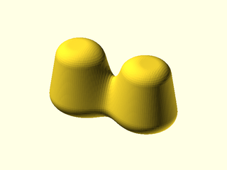
Example 3: Two rounded mb_cyl() cones interacting.
include <BOSL2/std.scad>
include <BOSL2/isosurface.scad>
spec = [
    left(10), mb_cyl(15, r1=6, r2=4, rounding=2),
    right(10), mb_cyl(15, r1=6, r2=4, rounding=2)
];
metaballs(spec, voxel_size=0.5,
    bounding_box=[[-17,-8,-10], [17,8,10]]);
Example 4: Two disks interacting. Here the arguments are in order and not named.
include <BOSL2/std.scad>
include <BOSL2/isosurface.scad>
metaballs([
    move([-10,0,2]), mb_disk(5,9),
    move([10,0,-2]), mb_disk(5,9)
    ], [[-20,-10,-6], [20,10,6]], 0.5);
Example 5: Two capsules interacting.

include <BOSL2/std.scad>
include <BOSL2/isosurface.scad>
metaballs([
    move([-8,0,4])*yrot(90), mb_capsule(16,3),
    move([8,0,-4])*yrot(90), mb_capsule(16,3)
    ], [[-17,-5,-8], [17,5,8]],  0.5);
Example 6: A sphere with two connectors.
include <BOSL2/std.scad>
include <BOSL2/isosurface.scad>
path = [[-20,0,0], [0,0,1], [0,-10,0]];
spec = [
    move(path[0]), mb_sphere(6),
    for(seg=pair(path)) each
       [IDENT, mb_connector(seg[0],seg[1],
        2, influence=0.5)]
];
metaballs(spec, voxel_size=0.5,
    bounding_box=[[-27,-13,-7], [4,7,14]]);
Example 7: Interaction between two tori in different orientations.
include <BOSL2/std.scad>
include <BOSL2/isosurface.scad>
spec = [
    move([-10,0,17]),        mb_torus(r_maj=6, r_min=2),
    move([7,6,21])*xrot(90), mb_torus(r_maj=7, r_min=3)
];
voxel_size = 0.5;
boundingbox = [[-19,-9,9], [18,10,32]];
metaballs(spec, boundingbox, voxel_size);
Example 8: Two octahedrons interacting. Here voxel_size is not given, so it defaults to a value that results in approximately 10,000 voxels in the bounding box. Adding the parameter show_stats=true displays the voxel size used, along with other information.
include <BOSL2/std.scad>
include <BOSL2/isosurface.scad>
metaballs([
    move([-11,0,4]), mb_octahedron(20),
    move([11,0,-4]), mb_octahedron(20)
    ], [[-21,-11,-14], [21,11,14]]);
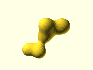
Example 9: These next five examples demonstrate the different types of metaball interactions. We start with two spheres 30 units apart. Each would have a radius of 10 in isolation, but because they are influencing their surroundings, each sphere mutually contributes to the size of the other. The sum of contributions between the spheres add up so that a surface plotted around the region exceeding the threshold defined by isovalue=1 looks like a peanut shape surrounding the two spheres.
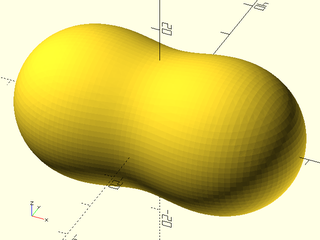
include <BOSL2/std.scad>
include <BOSL2/isosurface.scad>
spec = [
    left(15),  mb_sphere(10),
    right(15), mb_sphere(10)
];
voxel_size = 1;
boundingbox = [[-30,-19,-19], [30,19,19]];
metaballs(spec, boundingbox, voxel_size);
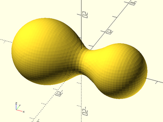
Example 10: Adding a cutoff of 25 to the left sphere causes its influence to disappear completely 25 units away (5 units from the center of the right sphere). The left sphere is bigger because it still receives the full influence of the right sphere, but the right sphere is smaller because the left sphere has no contribution past 25 units. The right sphere is not abruptly cut off because the cutoff function is smooth and influence is normal. Setting cutoff too small can remove the interactions of one metaball from all other metaballs, leaving that metaball alone by itself.

include <BOSL2/std.scad>
include <BOSL2/isosurface.scad>
spec = [
    left(15),  mb_sphere(10, cutoff=25),
    right(15), mb_sphere(10)
];
voxel_size = 1;
boundingbox = [[-30,-19,-19], [30,19,19]];
metaballs(spec, boundingbox, voxel_size);
Example 11: Here, the left sphere has less influence in addition to a cutoff. Setting influence=0.5 results in a steeper falloff of contribution from the left sphere. Each sphere has a different size and shape due to unequal contributions based on distance.
include <BOSL2/std.scad>
include <BOSL2/isosurface.scad>
spec = [
    left(15),  mb_sphere(10, influence=0.5, cutoff=25),
    right(15), mb_sphere(10)
];
voxel_size = 1;
boundingbox = [[-30,-19,-19], [30,19,19]];
metaballs(spec, boundingbox, voxel_size);
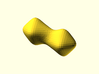
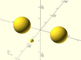
Example 12: In this example, we have two size-10 spheres as before and one tiny sphere of 1.5 units radius offset a bit on the y axis. With an isovalue of 1, this figure would appear similar to Example 9 above, but here the isovalue has been set to 2, causing the surface to shrink around a smaller volume values greater than 2. Remember, higher isovalue thresholds cause metaballs to shrink.
include <BOSL2/std.scad>
include <BOSL2/isosurface.scad>
spec = [
   left(15),  mb_sphere(10),
   right(15), mb_sphere(10),
   fwd(15),   mb_sphere(1.5)
];
voxel_size = 1;
boundingbox = [[-30,-19,-19], [30,19,19]];
metaballs(spec, boundingbox, voxel_size,
    isovalue=2);
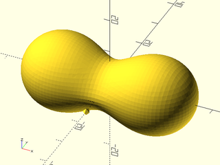
Example 13: Keeping isovalue=2, the influence of the tiny sphere has been set quite high, to 10. Notice that the tiny sphere shrinks a bit, but it has dramatically increased its contribution to its surroundings, causing the two other spheres to grow and meld into each other. The influence argument on a small metaball affects its surroundings more than itself.
include <BOSL2/std.scad>
include <BOSL2/isosurface.scad>
spec = [
   move([-15,0,0]), mb_sphere(10),
   move([15,0,0]),  mb_sphere(10),
   move([0,-15,0]), mb_sphere(1.5, influence=10)
];
voxel_size = 1;
boundingbox = [[-30,-19,-19], [30,19,19]];
metaballs(spec, boundingbox, voxel_size,
    isovalue=2);
Example 14: Setting influence to less than 0.5 can cause interpolation artifacts in the surface. The only difference between these two spheres is influence. Both have cutoff set to prevent them from affecting each other. The sphere on the right has a low influence of 0.02, which translates to a falloff with distance cutoff to limit the range of influence rather than reducing influence significantly below 1.

include <BOSL2/std.scad>
include <BOSL2/isosurface.scad>
spec = [
    left(10), mb_sphere(8, cutoff=10, influence=1),
    right(10), mb_sphere(8, cutoff=10, influence=0.02)
];
bbox = [[-18,-8,-8], [18,8,8]];
metaballs(spec, bounding_box=bbox, voxel_size=0.4);
Example 15: A group of five spherical metaballs with different sizes. The parameter show_stats=true (not shown here) was used to find a compact bounding box for this figure. Here instead of setting voxel_size, we set voxel_count for approximate number of voxels in the bounding box, and the voxel size is adjusted to fit. Setting exact_bounds=true forces the bounding box to be fixed, and a non-cubic voxel is then used to fit within that box.
include <BOSL2/std.scad>
include <BOSL2/isosurface.scad>
spec = [ // spheres of different sizes
    move([-20,-20,-20]), mb_sphere(5),
    move([0,-20,-20]),   mb_sphere(4),
    IDENT,               mb_sphere(3),
    move([0,0,20]),      mb_sphere(5),
    move([20,20,10]),    mb_sphere(7)
];
voxel_size = 1.5;
boundingbox = [[-30,-31,-31], [32,31,30]];
metaballs(spec, boundingbox,
    exact_bounds=true, voxel_count=40000);
Example 16: A metaball can be negative. In this case we have two metaballs in close proximity, with the small negative metaball creating a dent in the large positive one. The positive metaball is shown transparent, and small spheres show the center of each metaball. The negative metaball isn't visible because its field is negative; the isosurface encloses only field values greater than the isovalue of 1.

include <BOSL2/std.scad>
include <BOSL2/isosurface.scad>
centers = [[-1,0,0], [1.25,0,0]];
spec = [
    move(centers[0]), mb_sphere(8),
    move(centers[1]), mb_sphere(3, negative=true)
];
voxel_size = 0.25;
boundingbox = [[-7,-6,-6], [3,6,6]];
%metaballs(spec, boundingbox, voxel_size);
color("green") move_copies(centers) sphere(d=1, $fn=16);
Example 17: When a positive and negative metaball interact, the negative metaball reduces the influence of the positive one, causing it to shrink, but not disappear because its contribution approaches infinity at its center. In this example we have a large positive metaball near a small negative metaball at the origin. The negative ball has high influence, and a cutoff limiting its influence to 20 units. The negative metaball influences the positive one up to the cutoff, causing the positive metaball to appear smaller inside the cutoff range, and appear its normal size outside the cutoff range. The positive metaball has a small dimple at the origin (the center of the negative metaball) because it cannot overcome the infinite negative contribution of the negative metaball at the origin.
include <BOSL2/std.scad>
include <BOSL2/isosurface.scad>
spec = [
    back(10), mb_sphere(20),
    IDENT, mb_sphere(2, influence=30,
        cutoff=20, negative=true),
];
voxel_size = 0.5;
boundingbox = [[-20,-4,-20], [20,30,20]];
metaballs(spec, boundingbox, voxel_size);
Example 18: A sharp cube, a rounded cube, and a sharp octahedron interacting. Because the surface is generated through cubical voxels, voxel corners are always cut off, resulting in difficulty resolving some sharp edges.

include <BOSL2/std.scad>
include <BOSL2/isosurface.scad>
spec = [
    move([-7,-3,27])*zrot(55), mb_cuboid(6, squareness=1),
    move([5,5,21]),   mb_cuboid(5),
    move([10,0,10]),  mb_octahedron(10, squareness=1)
];
voxel_size = 0.5; // a bit slow at this resolution
boundingbox = [[-12,-9,3], [18,10,32]];
metaballs(spec, boundingbox, voxel_size);
Example 19: A toy airplane, constructed only from metaball spheres with scaling. The bounding box is used to clip the wingtips, tail, and belly of the fuselage.

include <BOSL2/std.scad>
include <BOSL2/isosurface.scad>
bounding_box = [[-55,-50,-5],[35,50,17]];
spec = [
    move([-20,0,0])*scale([25,4,4]),   mb_sphere(1), // fuselage
    move([30,0,5])*scale([4,0.5,8]),   mb_sphere(1), // vertical stabilizer
    move([30,0,0])*scale([4,15,0.5]),  mb_sphere(1), // horizontal stabilizer
    move([-15,0,0])*scale([6,45,0.5]), mb_sphere(1)  // wing
];
voxel_size = 1;
color("lightblue") metaballs(spec, bounding_box, voxel_size);
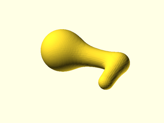
Example 20: Custom metaballs are an advanced technique in which you define your own metaball shape by passing a function literal that takes a single argument: a coordinate in space relative to the metaball center called point here, but can be given any name. This distance vector from the origin is calculated internally and always passed to the function. Inside the function, it is converted to a scalar distance dist. The function literal expression sets all of your parameters. Only point is not set, and it becomes the single parameter to the function literal. The spec argument invokes your custom function as a function literal that passes point into it.
include <BOSL2/std.scad>
include <BOSL2/isosurface.scad>
function threelobe(point) =
   let(
        ang=atan2(point.y, point.x),
        r=norm([point.x,point.y])*(1.3+cos(3*ang)),
        dist=norm([point.z, r])
   ) 3/dist;
metaballs(
    spec = [
        IDENT, function (point) threelobe(point),
        up(7), mb_sphere(r=4)
    ],
    bounding_box = [[-14,-12,-5],[8,12,13]],
    voxel_size=0.5);
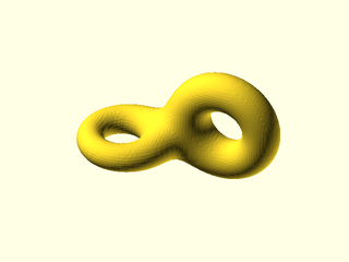
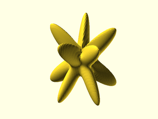
Example 21: Here is a function nearly identical to the previous example, introducing additional dimensional parameters into the function to control its size and number of lobes. The bounding box size here is as small as possible for calculation efficiency, but if you expiriment with this using different argument values, you should increase the bounding box along with voxel size.
include <BOSL2/std.scad>
include <BOSL2/isosurface.scad>
function multilobe(point, size, lobes) =
   let(
        ang=atan2(point.y, point.x),
        r=norm([point.x,point.y])*(1.3+cos(lobes*ang)),
        dist=norm([point.z, r])
   ) size/dist;
metaballs(
    spec = [
        left(7),
           function (point) multilobe(point, 3, 4),
        right(7)*zrot(60),
           function (point) multilobe(point, 3, 3)
    ],
    bounding_box = [[-16,-13,-5],[18,13,6]],
    voxel_size=0.4);
Example 22: Next we show how to create a function that works like the built-ins. This is a full-fledged implementation that allows you to specify the function directly by name in the spec argument without needing the function literal syntax, and without needing the point argument in spec, as in the prior examples. You must define a calculation function that accepts the point position argument and then whatever other parameters your metaball uses (here r and noise_level). Then there is a "master" function that does some error checking and returns a function literal expression that sets all of your parameters. The call to mb_cutoff() at the end handles the cutoff function for the noisy ball consistent with the other internal metaball functions; it requires dist and cutoff as arguments. You are not required to use this implementation in your own custom functions; in fact it's easier simply to declare the function literal in your spec argument, but this example shows how to do it all.
include <BOSL2/std.scad>
include <BOSL2/isosurface.scad>
//
// noisy sphere internal calculation function
function noisy_sphere_calcs(point, r, noise_level, cutoff, exponent, neg) =
let(
noise = rands(0, noise_level, 1)[0],
dist = norm(point) + noise
) neg * mb_cutoff(dist,cutoff) * (r/dist)^exponent;
// noisy sphere "master" entry function to use in spec argument
function noisy_sphere(r, noise_level, cutoff=INF, influence=1, negative=false, d) =
assert(is_num(cutoff) && cutoff>0, "\ncutoff must be a positive number.")
assert(is_finite(influence) && influence>0, "\ninfluence must be a positive number.")
let(
r = get_radius(r=r,d=d),
dummy=assert(is_finite(r) && r>0, "\ninvalid radius or diameter."),
neg = negative ? -1 : 1
) // pass control as a function literal to the calc function
function (point) noisy_sphere_calcs(point, r, noise_level, cutoff, 1/influence, neg);
// define the scene and render it
spec = [
left(9), mb_sphere(5),
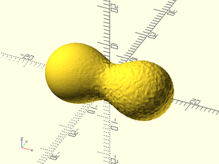
right(9), noisy_sphere(r=5, noise_level=0.2)
];
voxel_size = 0.5;
boundingbox = [[-16,-8,-8], [16,8,8]];
metaballs(spec, boundingbox, voxel_size);
Example 23: A more complex example using ellipsoids, a capsule, spheres, and a torus to make a tetrahedral object with rounded feet and a ring on top. The bottoms of the feet are flattened by clipping with the bottom of the bounding box. The center of the object is thick due to the contributions of three ellipsoids and a capsule converging. Designing an object like this using metaballs requires trial and error with low-resolution renders.

include <BOSL2/std.scad>
include <BOSL2/isosurface.scad>
include <BOSL2/polyhedra.scad>
tetpts = zrot(15, p = 22 * regular_polyhedron_info("vertices", "tetrahedron"));
tettransform = [ for(pt = tetpts) move(pt)*rot(from=RIGHT, to=pt)*scale([7,1.5,1.5]) ];

spec = [
    // vertical cylinder arm
    up(15), mb_capsule(17, 2, influence=0.8),
    // ellipsoid arms
    for(i=[0:2]) each [tettransform[i], mb_sphere(1, cutoff=30)],
    // ring on top
    up(35)*xrot(90), mb_torus(r_maj=8, r_min=2.5, cutoff=35),
    // feet
    for(i=[0:2]) each [move(2.2*tetpts[i]), mb_sphere(5, cutoff=30)],
];
voxel_size = 1;
boundingbox = [[-22,-32,-13], [36,32,46]];
// useful to save as VNF for copies and manipulations
vnf = metaballs(spec, boundingbox, voxel_size, isovalue=1);
vnf_polyhedron(vnf);
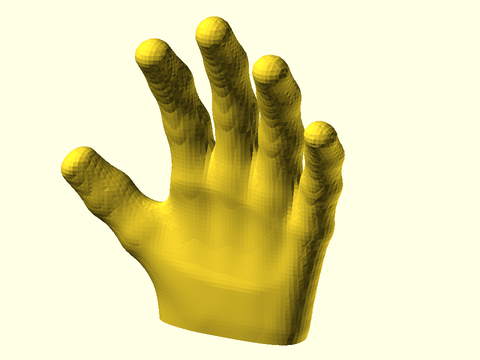
Example 24: This example demonstrates grouping metaballs together and nesting them in lists of other metaballs, to make a crude model of a hand. Here, just one finger is defined, and a thumb is defined from one less joint in the finger. Individual fingers are grouped together with different positions and scaling, along with the thumb. Finally, this group of all fingers is used to combine with a rounded cuboid, with a slight ellipsoid dent subtracted to hollow out the palm, to make the hand.
include <BOSL2/std.scad>
include <BOSL2/isosurface.scad>
joints = [[0,0,1], [0,0,85], [0,-5,125], [0,-16,157], [0,-30,178]];
finger = [
    for(i=[0:3]) each
        [IDENT, mb_connector(joints[i], joints[i+1], 9+i/5, influence=0.22)]
];
thumb = [
    for(i=[0:2]) each [
        scale([1,1,1.2]),
        mb_connector(joints[i], joints[i+1], 9+i/2, influence=0.28)
    ]
];
allfingers = [
    left(15)*zrot(5)*yrot(-50)*scale([1,1,0.6])*zrot(30), thumb,
    left(15)*yrot(-9)*scale([1,1,0.9]), finger,
    IDENT, finger,
    right(15)*yrot(8)*scale([1,1,0.92]), finger,
    right(30)*yrot(17)*scale([0.9,0.9,0.75]), finger
];
hand = [
    IDENT, allfingers,
    move([-5,0,5])*scale([1,0.36,1.55]), mb_cuboid(90, squareness=0.3, cutoff=80),
    move([-10,-95,50])*yrot(10)*scale([2,2,0.95]),
        mb_sphere(r=15, cutoff=50, influence=1.5, negative=true)
];
voxel_size=2.5;
bbox = [[-104,-40,-10], [79,18,188]];
metaballs(hand, bbox, voxel_size, isovalue=1);
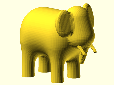
Example 25: A model of an elephant using cylinders, capsules, and disks.
include <BOSL2/std.scad>
include <BOSL2/isosurface.scad>
legD1 = 4.6;
legD2 = 1;
spec = [
    // legs
    up(1)*fwd(8)*left(13), mb_cyl(d1=legD1, d2=legD2, h=20),
    up(1)*fwd(8)*right(10), mb_cyl(d1=legD1, d2=legD2, h=20),
    up(1)*back(8)*left(13), mb_cyl(d1=legD1, d2=legD2, h=20),
    up(1)*back(8)*right(10), mb_cyl(d1=legD1, d2=legD2, h=20),
    up(20)*yrot(90), mb_capsule(d=21, h=36, influence=0.5), // body
    right(21)*up(25)*yrot(-20), mb_capsule(r=7, h=25, influence=0.5, cutoff=9), // head
    right(24)*up(10)*yrot(15), mb_cyl(d1=3, d2=6, h=15, cutoff=3), // trunk
    // ears
    right(18)*up(29)*fwd(11)*zrot(-20)*yrot(80)*scale([1.4,1,1]), mb_disk(r=5,h=2, cutoff=3),
    right(18)*up(29)*back(11)*zrot(20)*yrot(80)*scale([1.4,1,1]), mb_disk(r=5,h=2, cutoff=3),
    // tusks
    right(26)*up(13)*fwd(5)*yrot(135), mb_capsule(r=1, h=10, cutoff=1),
    right(26)*up(13)*back(5)*yrot(135), mb_capsule(r=1, h=10, cutoff=1)
];
bbox = [[-21,-17,-9], [31,17,38]];
metaballs(spec, bounding_box=bbox, voxel_size=1, isovalue=1);
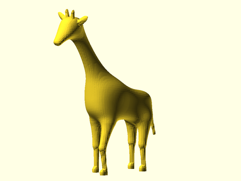
Example 26: A model of a giraffe using a variety of different metaball shapes. Features such as the tail and lower legs are thin, so a small voxel size is required to render them.
include <BOSL2/std.scad>
include <BOSL2/isosurface.scad>
legD = 1;
tibia = 14;
femur = 12;
head = [-35,0,78];  // head position
stance = [12,6];    // leg position offsets

spec = [
    // Legs
    move([-stance.x,-stance.y]), mb_connector([-4,0,0],[-6,0,tibia],legD, influence = 0.2),
    move([-stance.x,stance.y]),  mb_connector([0,0,0],[0,0,tibia],legD, influence = 0.2),
    move([stance.x,-stance.y]),  mb_connector([-2,0,0],[-3,0,tibia],legD, influence = 0.2),
    move([stance.x,stance.y]),   mb_connector([0,0,0],[0,0,tibia],legD, influence = 0.2),

    move([-stance.x,-stance.y,tibia]), mb_connector([-6,0,0],[-2,0,femur],legD),
    move([-stance.x,stance.y,tibia]),  mb_connector([0,0,0],[0,0,femur],legD),
    move([stance.x,-stance.y,tibia]),  mb_connector([-3,0,0],[-1,0,femur],legD),
    move([stance.x,stance.y,tibia]),   mb_connector([0,0,0],[0,0,femur],legD),

    // Hooves
    move([-stance.x-6,-stance.y,1]),    mb_capsule(d= 2, h = 3, cutoff = 2),
    move([-stance.x-1,stance.y,1]),     mb_capsule(d= 2, h = 3, cutoff = 2),
    move([stance.x-3.5,-stance.y,1]),   mb_capsule(d= 2, h = 3, cutoff = 2),
    move([stance.x-1,stance.y,1]),      mb_capsule(d= 2, h = 3, cutoff = 2),

    // Body
    up(tibia+femur+10) * yrot(10),        mb_cuboid([16,7,7]),
    up(tibia+femur+15)*left(10),          mb_sphere(2),
    up(tibia+femur+8)*right(13)*xrot(90), mb_disk(1,4),

    // Tail
    up(tibia+femur+8), mb_connector([18,0,0],[22,0,-16], 0.4, cutoff = 1),

    // Neck
    up(tibia+femur+35)*left(22)*yrot(-30)* yscale(0.75), mb_cyl(d1 = 5, d2 = 3, l = 38),

    // Head
    move(head + [-4,0,-3])*yrot(45)*xscale(0.75), mb_cyl(d1 = 1.5, d2 = 4, l = 12, rounding=0),
    move(head), mb_cuboid(2),

    // Horns
    move(head), mb_connector([0,-2,5],[0,-2.5,8],0.3, cutoff = 1),
    move(head + [0,-2.5,8]), mb_sphere(0.5, cutoff = 1),
    move(head), mb_connector([0,2,5],[0,2.5,8],0.3, cutoff = 1),
    move(head + [0,2.5,8]), mb_sphere(0.5, cutoff = 1),

    // Ears
    move(head + [2,-8,4])* xrot(60) * scale([0.5,1,3]) , mb_sphere(d = 2, cutoff = 2),
    move(head + [2,8,4])* xrot(-60) * scale([0.5,1,3]) , mb_sphere(d = 2, cutoff = 2),
];
vsize = 0.85;
bbox =  [[-45.5, -11.5, 0], [23, 11.5, 87.55]];
metaballs(spec, bbox, voxel_size=vsize);
Example 27: A model of a bunny, made from separate body components made with metaballs, with each component rendered at a different voxel size, and then combined together along with eyes and teeth. In this way, smaller bounding boxes can be defined for each component, which speeds up rendering. A bit more time is saved by saving the repeated components (ear, front leg, hind leg) in VNF structures, to render copies with vnf_polyhedron().
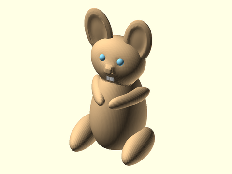
include <BOSL2/std.scad>
include <BOSL2/isosurface.scad>
torso = [
    up(20) * scale([1,1.2,2]), mb_sphere(10),
    up(10), mb_sphere(5) // fatten lower torso
];
head = [
    up(50) * scale([1.2,0.8,1]), mb_sphere(10, cutoff = 15),
    // nose
    move([0,-11,50]), mb_cuboid(2),
    // eye sockets
    move([5,-10,54]), mb_sphere(0.5, negative = true),
    move([-5,-10,54]), mb_sphere(0.5, negative = true),
    // tail
    move([0,15,6]), mb_sphere(2, cutoff = 5)
];
hind_leg = [
    move([-15,-5,3]) * scale([1.5,4,1.75]), mb_sphere(5),
    move([-15,10,3]), mb_sphere(3, negative = true)
];
front_leg = [
    move([-9,-4,30]) * zrot(30) * scale([1.5,5,1.75]), mb_sphere(3),
    move([-9,10,30]), mb_sphere(2, negative = true)
];
ear = [
    yrot(10) * move([0,0,65]) * scale([4,1,7]), mb_sphere(2),
    yrot(10)*move([0,-3,65])*scale([3,2,6]), mb_sphere(2, cutoff = 2, influence =2, negative = true)
];
vnf_hindleg = metaballs(hind_leg, [[-22,-24,0],[-8,7,11]], voxel_size=0.8);
vnf_frontleg = metaballs(front_leg, [[-16,-17,25], [-1,7,35]], voxel_size=0.6);
vnf_ear = metaballs(ear, [[3,-2,50],[20,2,78]], voxel_size=0.6);
color("BurlyWood") {
    metaballs([IDENT, torso, IDENT, head],
        [[-16,-17,0],[16,20,63]], voxel_size=0.7);
    xflip_copy() {
        vnf_polyhedron(vnf_hindleg);
        vnf_polyhedron(vnf_frontleg);
        vnf_polyhedron(vnf_ear);;
    }
}
// add eyes
xflip_copy() move([5,-8,54]) color("skyblue") sphere(2, $fn = 32);
// add teeth
xflip_copy() move([1.1,-10,44]) color("white") cuboid([2,0.5,4], rounding = 0.15);
Synopsis: Creates a 3D isosurface (a 3D contour) from a function or array of values. [Geom] [VNF]
Topics: Isosurfaces, VNF Generators
Usage: As a module
- isosurface(f, isovalue, bounding_box, voxel_size, [voxel_count=], [reverse=], [closed=], [exact_bounds=], [show_stats=], ...) [ATTACHMENTS];
Usage: As a function
- vnf = isosurface(f, isovalue, bounding_box, voxel_size, [voxel_count=], [reverse=], [closed=], [exact_bounds=], [show_stats=]);
Description:
Computes a VNF structure of an object bounded by an isosurface or a range between two isosurfaces, within a specified bounding box.
The isosurface of a function [x,y,z] coordinate as input to define the grid coordinate location and
returning a single numerical value.
You can also define an isosurface using a 3D array of values instead of a function, in which
case the isosurface is the set of points equal to the isovalue as interpolated from the array.
The array indices are in the order [x][y][z].
The isovalue must be specified as a range [c_min,c_max]. The range can be finite or unbounded at one
end, with either c_min=-INF or c_max=INF. The returned object is the set of points [x,y,z] that
satisfy c_min <= f(x,y,z) <= c_max. If f(x,y,z) has values larger than c_min and values smaller than
c_max, then the result is a shell object with two bounding surfaces corresponding to the
isosurfaces at c_min and c_max. If f(x,y,z) < c_max
everywhere (which is true when c_max = INF), then no isosurface exists for c_max, so the object
has only one bounding surface: the one defined by c_min. This can result in a bounded object
like a sphere, or it can result an an unbounded object such as all the points outside of a sphere out
to infinity. A similar situation arises if f(x,y,z) > c_min everywhere (which is true when
c_min = -INF). Setting isovalue to [-INF,c_max] or [c_min,INF] always produces an object with a
single bounding isosurface, which itself can be unbounded. To obtain a bounded object, think about
whether the function values inside your object are smaller or larger than your isosurface value. If
the values inside are smaller, you produce a bounded object using [-INF,c_max]. If the values
inside are larger, you get a bounded object using [c_min,INF].
The isosurface is evaluated over a bounding box, which can be a scalar cube, or specified by its
minimum and maximum corners [[xmin,ymin,zmin],[xmax,ymax,zmax]]. This bounding box is divided into
voxels of the specified voxel_size, which can also be a scalar cube, or a vector size. Smaller
voxels produce a finer, smoother result at the expense of execution time. By default, if the voxel
size doesn't exactly divide your specified bounding box, then the bounding box is enlarged to
contain whole voxels, and centered on your requested box. Alternatively, you may set
exact_bounds=true to force the voxels to adjust in size to fit instead.
Either way, if the bounding box clips the isosurface and closed=true (the default), a surface is
added to create a closed manifold object. Setting closed=false causes the VNF faces to end at the
bounding box, resulting in a non-manifold shape that exposes the inside of the object.
Why does my object appear as a cube? If your object is unbounded, then when it intersects with
the bounding box and closed=true, the result may appear to be a solid cube, because the clipping
faces are all you can see and the bounding surface is hidden inside. Setting closed=false removes
the bounding box faces and exposes the inside structure (with inverted faces). If you want the bounded
object, you can correct this problem by changing your isovalue range. If you were using a finite range
[c1,c2], try changing it to [c2,INF] or [-INF,c1]. If you were using an unbounded range like
[c,INF], try switching the range to [-INF,c].
Run time: The size of the voxels and size of the bounding box affects the run time, which can be long.
A voxel size of 1 with a bounding box volume of 200×200×200 may be slow because it requires the
calculation and storage of 8,000,000 function values, and more processing and memory to generate
the triangulated mesh. On the other hand, a voxel size of 5 over a 100×100×100 bounding box
requires only 8,000 function values and a modest computation time. A good rule is to keep the number
of voxels below 10,000 for preview, and adjust the voxel size smaller for final rendering. If you don't
specify voxel_size or voxel_count then metaballs uses a default voxel_count of 10000, which should be
reasonable for initial preview. Because a bounding
box that is too large wastes time computing function values that are not needed, you can also set the
parameter show_stats=true to get the actual bounds of the voxels intersected by the surface. With this
information, you may be able to decrease run time, or keep the same run time but increase the resolution.
Manifold warnings: The point list in the generated VNF structure contains many duplicated points. This is normally not a
problem for rendering the shape, but machine roundoff differences may result in Manifold issuing
warnings when doing the final render, causing rendering to abort if you have enabled the "stop on
first warning" setting. You can prevent this by passing the VNF through vnf_quantize() using a
quantization of 1e-7, or you can pass the VNF structure into vnf_merge_points(), which also
removes the duplicates. Additionally, flat surfaces (often resulting from clipping by the bounding
box) are triangulated at the voxel size resolution, and these can be unified into a single face by
passing the vnf structure to vnf_unify_faces(). These steps can be computationally expensive
and are not normally necessary.
Arguments:
| By Position | What it does |
|---|---|
f |
The isosurface function literal or array. As a function literal, x,y,z must be the first arguments. |
isovalue |
A 2-vector giving an isovalue range. For an unbounded range, use [-INF, max_isovalue] or [min_isovalue, INF]. |
bounding_box |
The volume in which to perform computations, expressed as a scalar size of a cube centered on the origin, or a pair of 3D points [[xmin,ymin,zmin], [xmax,ymax,zmax]] specifying the minimum and maximum box corner coordinates. Unless you set exact_bounds=true, the bounding box size may be enlarged to fit whole voxels. When f is an array of values, bounding_box cannot be supplied if voxel_size is supplied because the bounding box is already implied by the array size combined with voxel_size, in which case this implied bounding box is centered around the origin. |
voxel_size |
Size of the voxels used to sample the bounding box volume, can be a scalar or 3-vector, or omitted if voxel_count is set. You may get a non-cubical voxels of a slightly different size than requested if exact_bounds=true. |
| By Name | What it does |
|---|---|
voxel_count |
Approximate number of voxels in the bounding box. If exact_bounds=true then the voxels may not be cubes. Use with show_stats=true to see the corresponding voxel size. Default: 10000 (if voxel_size not set) |
closed |
When true, close the surface if it intersects the bounding box by adding a closing face. When false, do not add a closing face and instead produce a non-manfold VNF that has holes. Default: true |
reverse |
When true, reverses the orientation of the VNF faces. Default: false |
exact_bounds |
When true, shrinks voxels as needed to fit whole voxels inside the requested bounding box. When false, enlarges bounding_box as needed to fit whole voxels of voxel_size, and centers the new bounding box over the requested box. Default: false |
show_stats |
If true, display statistics in the console window about the isosurface: number of voxels that the surface passes through, number of triangles, bounding box of the voxels, and voxel-rounded bounding box of the surface, which may help you reduce your bounding box to improve speed. Enabling this parameter has a slight speed penalty. Default: false |
show_box |
(Module only) display the requested bounding box as transparent. This box may appear slightly inside the bounds of the figure if the actual bounding box had to be expanded to accommodate whole voxels. Default: false |
convexity |
(Module only) Maximum number of times a line could intersect a wall of the shape. Affects preview only. Default: 6 |
cp |
(Module only) Center point for determining intersection anchors or centering the shape. Determines the base of the anchor vector. Can be "centroid", "mean", "box" or a 3D point. Default: "centroid" |
anchor |
(Module only) Translate so anchor point is at origin (0,0,0). See anchor. Default: "origin"
|
spin |
(Module only) Rotate this many degrees around the Z axis after anchor. See spin. Default: 0
|
orient |
(Module only) Vector to rotate top toward, after spin. See orient. Default: UP
|
atype |
(Module only) Select "hull" or "intersect" anchor type. Default: "hull" |
Anchor Types:
| Anchor Type | What it is |
|---|---|
| "hull" | Anchors to the virtual convex hull of the shape. |
| "intersect" | Anchors to the surface of the shape. |
Named Anchors:
| Anchor Name | Position |
|---|---|
| "origin" | Anchor at the origin, oriented UP. |
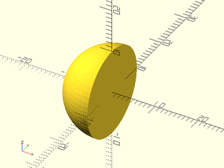
Example 1: These first three examples demonstrate the effect of isovalue range for the simplest of all surfaces: a sphere where r = norm([x,y,z]) in OpenSCAD. Then, the isosurface corresponding to an isovalue of 10 is every point where the expression norm([x,y,z]) equals a radius of 10. We use the isovalue range [-INF,10] here to make the sphere, with a bounding box that cuts off half the sphere. The isovalue range could also be [0,10] because the minimum value of the expression is zero.
include <BOSL2/std.scad>
include <BOSL2/isosurface.scad>
isovalue = [-INF,10];
bbox = [[-11,-11,-11], [0,11,11]];
isosurface(function (x,y,z) norm([x,y,z]),
   isovalue, bbox, voxel_size = 1);
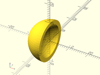
Example 2: An isovalue range [8,10] gives a shell with inner radius 8 and outer radius 10.
include <BOSL2/std.scad>
include <BOSL2/isosurface.scad>
isovalue = [8,10];
bbox = [[-11,-11,-11], [0,11,11]];
isosurface(function (x,y,z) norm([x,y,z]),
   isovalue, bbox, voxel_size = 1);
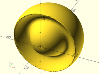
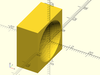
Example 3: Here we set the isovalue range to [10,INF]. Because the sphere expression norm(xyz) has larger values growing to infinity with distance from the origin, the resulting object appears as the bounding box with a radius-10 spherical hole.
include <BOSL2/std.scad>
include <BOSL2/isosurface.scad>
isovalue = [10,INF];
bbox = [[-11,-11,-11], [0,11,11]];
isosurface(function (x,y,z) norm([x,y,z]),
   isovalue, bbox, voxel_size = 1);
Example 4: Unlike a sphere, a gyroid is unbounded; it's an isosurface defined by all the zero values of a 3D periodic function. To illustrate what the surface looks like, closed=false has been set to expose both sides of the surface. The surface is periodic and tileable along all three axis directions. This is a non-manifold surface as displayed, not useful for 3D modeling. This example also demonstrates using an additional parameter in the field function beyond just the [x,y,z] input; in this case to control the wavelength of the gyroid.

include <BOSL2/std.scad>
include <BOSL2/isosurface.scad>
function gyroid(x,y,z, wavelength) = let(
    p = 360/wavelength * [x,y,z]
) sin(p.x)*cos(p.y)+sin(p.y)*cos(p.z)+sin(p.z)*cos(p.x);
isovalue = [0,INF];
bbox = [[-100,-100,-100], [100,100,100]];
isosurface(function(x,y,z) gyroid(x,y,z, wavelength=200),
    isovalue, bbox, voxel_size=5, closed=false);
Example 5: If we remove the closed parameter or set it to true, the isosurface algorithm encloses the entire half-space bounded by the "inner" gyroid surface, leaving only the "outer" surface exposed. This is a manifold shape but not what we want if trying to model a gyroid.
include <BOSL2/std.scad>
include <BOSL2/isosurface.scad>
function gyroid(x,y,z, wavelength) = let(
    p = 360/wavelength * [x,y,z]
) sin(p.x)*cos(p.y)+sin(p.y)*cos(p.z)+sin(p.z)*cos(p.x);
isovalue = [0,INF];
bbox = [[-100,-100,-100], [100,100,100]];
isosurface(function(x,y,z) gyroid(x,y,z, wavelength=200),
    isovalue, bbox, voxel_size=5, closed=true);
Example 6: To make the gyroid a double-sided surface, we need to specify a small range around zero for isovalue. Now we have a double-sided surface although with closed=false the edges are not closed where the surface is clipped by the bounding box.

include <BOSL2/std.scad>
include <BOSL2/isosurface.scad>
function gyroid(x,y,z, wavelength) = let(
    p = 360/wavelength * [x,y,z]
) sin(p.x)*cos(p.y)+sin(p.y)*cos(p.z)+sin(p.z)*cos(p.x);
isovalue = [-0.3, 0.3];
bbox = [[-100,-100,-100], [100,100,100]];
isosurface(function(x,y,z) gyroid(x,y,z, wavelength=200),
    isovalue, bbox, voxel_size=5, closed=false);
Example 7: To make the gyroid a valid manifold 3D object, we remove the closed parameter (same as setting closed=true), which closes the edges where the surface is clipped by the bounding box.

include <BOSL2/std.scad>
include <BOSL2/isosurface.scad>
function gyroid(x,y,z, wavelength) = let(
    p = 360/wavelength * [x,y,z]
) sin(p.x)*cos(p.y)+sin(p.y)*cos(p.z)+sin(p.z)*cos(p.x);
isovalue = [-0.3, 0.3];
bbox = [[-100,-100,-100], [100,100,100]];
isosurface(function(x,y,z) gyroid(x,y,z, wavelength=200),
    isovalue, bbox, voxel_size=5);
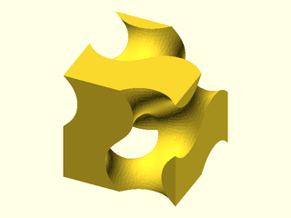
Example 8: An approximation of the triply-periodic minimal surface known as Schwartz P.

include <BOSL2/std.scad>
include <BOSL2/isosurface.scad>
function schwartz_p(x,y,z, wavelength) = let(
    p = 360/wavelength,
    px = p*x, py = p*y, pz = p*z
)  cos(px) + cos(py) + cos(pz);
isovalue = [-0.2, 0.2];
bbox = [[-100,-100,-100], [100,100,100]];
isosurface(function (x,y,z) schwartz_p(x,y,z, 100),
    isovalue, bounding_box=bbox, voxel_size=4);
Example 9: Another approximation of the triply-periodic minimal surface known as Neovius.

include <BOSL2/std.scad>
include <BOSL2/isosurface.scad>
function neovius(x,y,z, wavelength) = let(
    p = 360/wavelength,
    px = p*x, py = p*y, pz = p*z
)  3*(cos(px) + cos(py) + cos(pz)) + 4*cos(px)*cos(py)*cos(pz);
bbox = [[-100,-100,-100], [100,100,100]];
isosurface(function (x,y,z) neovius(x,y,z, 200),
    isovalue = [-0.3, 0.3],
    bounding_box = bbox, voxel_size=4);
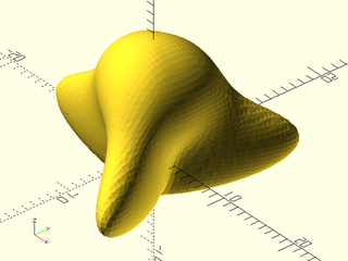
Example 10: Example of a bounded isosurface.
include <BOSL2/std.scad>
include <BOSL2/isosurface.scad>
isosurface(
    function (x,y,z)
        let(a=xyz_to_spherical([x,y,z]),
            r=a[0],
            phi=a[1],
            theta=a[2]
        ) 1/(r*(3+cos(5*phi)+cos(4*theta))),
    isovalue = [0.1,INF],
    bounding_box = [[-8,-7,-8],[6,7,8]],
    voxel_size = 0.25);
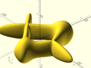
Example 11: Another example of a bounded isosurface.

include <BOSL2/std.scad>
include <BOSL2/isosurface.scad>
isosurface(function (x,y,z)
      2*(x^4 - 2*x*x + y^4
         - 2*y*y + z^4 - 2*z*z) + 3,
    bounding_box=3, voxel_size=0.07,
    isovalue=[-INF,0]);
Example 12: For shapes that occupy a cubical bounding box centered on the origin, you can simply specify a scalar for the size of the box.

include <BOSL2/std.scad>
include <BOSL2/isosurface.scad>
isosurface(
    function (x,y,z) let(np=norm([x,y,z]))
       (x*y*z^3 + 19*x^2*z^2) / np^2 + np^2,
    isovalue=[-INF,35], bounding_box=12, voxel_size=0.25);
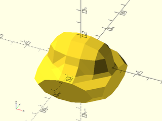
Example 13: An object that could be a sort of support pillar. Here we set show_box=true to reveal that the bounding box is slightly bigger than it needs to be. The argument show_stats=true also outputs the voxel bounding box size as a suggestion of what it should be.

include <BOSL2/std.scad>
include <BOSL2/isosurface.scad>
isosurface(
    function (x,y,z) let(np=norm([x,y,z]))
       (x*y*z^3 - 3*x^2*z^2) / np^2 + np^2,
    isovalue=[-INF,35], bounding_box=[[-32,-32,-14],[32,32,14]],
    voxel_size = 0.8, show_box=true);
Example 14: You can specify non-cubical voxels for efficiency. This example shows the result of two identical surface functions. The figure on the left uses a voxel_size=1, which washes out the detail in the z direction. The figure on the right shows the same shape with voxel_size=[0.5,1,0.2] to give a bit more resolution in the x direction and much more resolution in the z direction. This example runs about six times faster than if we used a cubical voxel of size 0.2 to capture the detail in only one axis at the expense of unnecessary detail in other axes.

include <BOSL2/std.scad>
include <BOSL2/isosurface.scad>
function shape(x,y,z, r=5) =
    r / sqrt(x^2 + 0.5*(y^2 + z^2) + 0.5*r*cos(200*z));
bbox = [[-6,-8,0], [6,8,7]];

left(6) isosurface(function (x,y,z) shape(x,y,z),
    isovalue=[1,INF], bounding_box=bbox, voxel_size=1);

right(6) isosurface(function (x,y,z) shape(x,y,z),
    isovalue=[1,INF], bounding_box=bbox, voxel_size=[0.5,1,0.2]);
Example 15: Nonlinear functions with steep gradients between voxel corners at the isosurface value can show interpolation ridges because the surface position is approximated by a linear interpolation of a highly nonlinear function. The appearance of the artifacts depends on the combination of function, voxel size, and isovalue, and can look different in different circumstances. If your isovalue is positive, then you may be able to smooth out the artifacts by using the log of your function and the log of your isovalue range to get the same isosurface without artifacts. On the left, an isosurface around a steep nonlinear function (clipped on the left by the bounding box) exhibits severe interpolation artifacts. On the right, the log of the isosurface around the log of the function smooths it out nicely.

include <BOSL2/std.scad>
include <BOSL2/isosurface.scad>
bbox = [[0,-10,-5],[9,10,6]];

function shape(x,y,z) =
        exp(-((x+5)/5-3)^2-y^2)
        *exp(-((x+5)/3)^2-y^2-z^2)
        + exp(-((y+4)/5-3)^2-x^2)
        *exp(-((y+4)/3)^2-x^2-0.5*z^2);

left(6) isosurface(function(x,y,z) shape(x,y,z),
    isovalue = [EPSILON,INF],
    bounding_box=bbox, voxel_size=0.25);
right(6) isosurface(function(x,y,z) log(shape(x,y,z)),
    isovalue = [log(EPSILON),INF],
    bounding_box=bbox, voxel_size=0.25);
Example 16: Using an array for the f argument instead of a function literal. Each row of the array represents an X index for a YZ plane with the array Z indices changing fastest in each plane. The final object may need rotation to get the orientation you want. You don't pass the bounding_box argument here; it is implied by the array size and voxel size, and centered on the origin.
include <BOSL2/std.scad>
include <BOSL2/isosurface.scad>
field = [
  repeat(0,[6,6]),
  [ [0,1,2,2,1,0],
    [1,2,3,3,2,1],
    [2,3,4,4,3,2],
    [2,3,4,4,3,2],
    [1,2,3,3,2,1],
    [0,1,2,2,1,0]
  ],
  [ [0,0,0,0,0,0],
    [0,0,1,1,0,0],
    [0,2,3,3,2,0],
    [0,2,3,3,2,0],
    [0,0,1,1,0,0],
    [0,0,0,0,0,0]
  ],
  [ [0,0,0,0,0,0],
    [0,0,0,0,0,0],
    [0,1,2,2,1,0],
    [0,1,2,2,1,0],
    [0,0,0,0,0,0],
    [0,0,0,0,0,0]
  ],
  repeat(0,[6,6])
];
rotate([0,-90,180])
   isosurface(field, isovalue=[0.5,INF],
       voxel_size=10);